Control based on Function Approximation

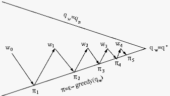
The control algorithms based on approximated value functions also follow the general method of the general policy iteration, as illustrated bellow:

We note that this is similar to the algorithms for model-free control illustrated in Fig. 1.4, but with the action-value function $q_\pi(s,a)$ is replaced by the parameter ${\bf w}$ of the approximation action function $\hat{q}(s,a,{\bf w})$. In particular, for a linear function, we have:

$$\hat{q}(s,a,{\bf w})=\sum_nw_nx(s,a)={\bf w}^T{\bf x}_n(s,a)$$ (94)

where ${\bf x}(s,a)$ is the feature vector for the state-action pair $(s,a)$. We need to find the optimal parameter ${\bf w}$ that minimizes the objective function, the mean square error of the approximation:

$$J({\bf w}) =\frac{1}{2}E_\pi[(q_\pi(s,a)-\hat{q}(s,a,{\bf w}))^2] =\frac{1}{2}E_\pi[(q_\pi(s,a)-{\bf w}^T{\bf x}(s,a))^2]$$ (95)

with gradient vector:

$$\triangledown J({\bf w}) = \frac{d}{d{\bf w}}J({\bf w}) =-E_\pi\left[q_\pi(s,a)-\hat{q}(s,a,{\bf w})\right] \triangledown\hat{q}(s,a,{\bf w})$$

$$= -E_\pi\left[(q_\pi(s,a)-{\bf w}^T{\bf x}(s,a)){\bf x}(s,a)\right]$$ (96)

If the stochastic gradient descent method is used based on a single sample of the action value $q_\pi(s,a)$, instead of its expectation, then $E_\pi$ can be dropped, and the optimal weight vector ${\bf w}^*$ that minimizes $J({\bf w})$ in Eq. (95) can be learned iteratively:

$${\bf w}_{t+1} = {\bf w}_t+\Delta{\bf w} ={\bf w}_t-\alpha\triangledown{\bf J}({\bf w})$$

$$= {\bf w}_t+\alpha\left[(q_\pi(s_t,a_t)-\hat{q}_\pi(s_t,a_t,{\bf w})) \triangledown\hat{q}_\pi(s_t,a_t,{\bf w}) \right]$$

$$= {\bf w}_t+\alpha\left[(q_\pi(s_t,a_t)-{\bf w}_t^T{\bf x}(s_t,a_t)) {\bf x}(s_t,a_t) \right]$$ (97)

where $\Delta{\bf w}$ is the increment of the update:

$$\Delta{\bf w}=-\alpha\triangledown{\bf J}({\bf w}) = \alpha[ q_\pi(s_t,a_t)-\hat{q}_\pi(s_t,a_t,{\bf w})] \triangledown\hat{q}_\pi(s_t,a_t,{\bf w})$$

$$= \alpha[ q_\pi(s_t,a_t)-{\bf w}_t^T{\bf x}(s_t,a_t) ] {\bf x}(s_t,a_t)$$ (98)

As the true Q-value $q_\pi(s,a)$ in the expression is unknown, it needs to be estimated by some target depending on the specific methods used:

• MC method:

  The true $q_\pi(s,a)$ is replaced by the sample return $G_t$ as the target, obtained at the end of each episode:

  $$\Delta{\bf w} =\alpha[G_t-\hat{q}(s_t,a_t,{\bf w})] \triangledown \hat{q}(s_t,a_t,{\bf w}) =\alpha[G_t-{\bf w}_t^T{\bf x}(s_t,a_t)]{\bf x}(s_t,a_t)$$ (99)

• TD(0) method:

  The action value function $q_\pi(s,a)$ is replaced by the TD target, the sum of the immediate reward, available at each step of each spisode, and the approximated action value of the next state $s_{t+1}$:

  • SARSA (on-policy):
    

    $$\Delta{\bf w} = \alpha[r_{t+1}+\gamma\hat{q}(s_{t+1},a_{t+1},{\bf w}) -\hat{q}(s_t,a_t,{\bf w}) ] \triangledown\hat{q}(s_t,a_t,{\bf w})$$

    $$= \alpha[r_{t+1}+\gamma{\bf w}^T{\bf x}(s_{t+1},a_{t+1}) -{\bf w}_t^T{\bf x}(s_t,a_t) ]{\bf x}(s_t,a_t)$$ (100)

    
    

    Following Eq. (71), the TD error is defined as:

    $$\delta_t=r_{t+1}+\gamma\hat{q}(s_{t+1},a_{t+1},{\bf w}) -\hat{q}(s_t,a_t,{\bf w})$$ (101)

    then we get

    $$\Delta{\bf w}=\alpha\delta_t \triangledown\hat{q}(s_t,a_t,{\bf w})$$ (102)

  • Q-learning (off-policy):
    

    $$\Delta{\bf w} = \alpha[r_{t+1}+\gamma\max_{a'} \hat{q}(s_{t+1},a',{\bf w})-\hat{q}(s_t,a_t,{\bf w}) ] \triangledown\hat{q}(s_t,a_t,{\bf w})$$

    $$= \alpha[r_{t+1}+\gamma\max_{a'} {\bf w}^T{\bf x}(s_{t+1},a')-{\bf w}_t^T{\bf x}(s_t,a_t)]{\bf x}(s,a)$$ (103)

    
    

• TD($\lambda$) method:

  In the forward-view version of the TD($\lambda$) method the action function $q_\pi(s,a)$ is approximated by $\lambda$-return $G_t^\lambda$ as the target, available only at the end of each spisode:

  $$\Delta{\bf w} =\alpha[ G_t^\lambda-{\bf w}_t^T{\bf x}(s_t,a_t) ]{\bf x}(s_t,a_t)$$ (104)

  The backward-view version of the TD($\lambda$) method based on eligibility traces is more advantageous in both space and temporal complexity as well as learning efficiency.

  We first define an eligiibility trace vector which is set to zero at the beginning of the episode, but then decays

  $$e_t=\gamma\lambda e_{t-1}+\triangledown_w\hat{q}(s_t,a_t,{\bf w})$$ (105)

  $$\Delta{\bf w}=\alpha\delta_te_t$$ (106)

  and Eq. (70)

  $$v_\pi(s)=v_\pi(s)+\alpha\delta_te_t(s),\;\;\;\;\;\;\; \forall s\in S$$ (107)

  /////

  Recall the TD error for the backward view of the TD($\lambda$) method first given in Eq. (71):

  $$\delta_t=(r_{t+1}+\gamma v_\pi(s_{t+1})-v_\pi(s))$$ (108)

In summary, here are the conceptual (not necessarily algorithmic) steps for the general model-free control based on approximated action-value function:

• Learn parameter ${\bf w}$ as in Eq. (97),
• Get the Q-values as in Eq. (94)
• Obtain the policy by $\epsilon$-greedy approach as in Eq. (41)

These steps are also illustrated below:

$$\mbox{Training of ${\bf w}$} \Longrightarrow Q-value \Longrightarrow \mbox{Policy $\pi$}$$ (109)