Autoencoder

Autoencoder is a neural network method that learns to represent the patterns in a given dataset in such a way that both the dimensionality and the noise are reduced. An autoencoder is similar to the back propogation network in that it is composed of an input layer that takes the input pattern ${\bf x}$, one or more hidden (latent) layers, and an output layer with the same number of nodes that generates an output $\hat{\bf x}$ as a represention of the current input ${\bf x}$. Different from a back propogation network that learns to associate a pattern ${\bf x}_i$ to the corresponding pattern ${\bf y}_i$, the labeling as a function of ${\bf x}_i$, the autoencoder is an unsupervised learning method based on unlabeled dataset, that learns to associate each pattern ${\bf x}_i$ to itself, i.e., an identify function. However, the purpose of the autoencoder is not to simply copy the data, instead, by imposing constraints such as sparsity to the hidden layer(s) in terms of the number of nodes or the number of activated nodes, the hidden layer becomes the bottleneck of the multi-layer network that represents the essential information in the data in terms of activation of the hidden layer nodes, the code. As, typically the number of hidden layer nodes is much smaller than those in the input and output layers, the input patterns that are reconstructed by the output of the network are encoded by the hidden layer nodes in a lower dimensional space. As the result, the autoencoder is forced to represent the data in reduced data size for data compression, if the components of ${\bf x}$ in the dataset are correlated, and to discover potential structures in the dataset.

An autoencoder is similar to the PCA algorithm in that both can extract essential information from the data and thereby compress the data without losing information. However, the PCA does this in a linear manner as its output principal components are linear combinations of the input signal components, but the components generated by the hidden layer nodes of an autoencoder are nonlinear functions (due to the activation function) of the input signal components. This nonlinearity makes an autoencoder more powerful.

The computation taking place in an autoencoder can be considered as an encoding/decoding process. The encoder is composed of an encoder composed of the input layer and the hidden layers, and a decoder is composed of the hidden layers and the output layer. Same as in back propogation, a pattern vector ${\bf x}$ presented to the input layer is forward propogated first to the hidden layer by

$$z_j=g\left(\sum_{k=0}^d w^h_{jk}x_k\right)\;\;\;\;\;(j=1,\cdots,l) \;\;\;\;\;\;\;\; {\bf z}={\bf g}({\bf W}^h{\bf x})$$ (66)

same as in Eq. (47), and then further to the output layer by

$$\hat{x}_i=g\left(\sum_{j=0}^l w^o_{ij}z_k\right)\;\;\;\;\;(i=1,\cdots,m) \;\;\;\;\;\;\;\; \hat{\bf x}={\bf g}({\bf W}^o{\bf z})$$ (67)

same as in Eq. (49). Also same as in back propogation, the weigths in both ${\bf W}^h$ and ${\bf W}^o$ are updated during training in the back propogation process so that the following objective function for the squared error between the input and desired output, the same as the input, is minimized:

$$\varepsilon=\frac{1}{2}\vert\vert{\bf x}-\hat{\bf x}\vert\vert^2$$ (68)

Here we assume there is only a single hidden layer for convenicne, but the computation for both the forward and backward passes can be easily extended to multiple layers.

By limiting the number $l$ of the hidden layer(s) to be smaller than that of input and output layer, the dimensionality of the data can be reduced from $d$ for the dimensionality of the input ${\bf x}=[x_1,\cdots,x_d]^T$ to $l$, the number of hidden layer nodes, while most of the information in the original data is reserved.

It is interesting to compare the autoencoder and the KLT transform in terms of how they map a given data vector ${\bf x}$ in the original d-dimensional space to a lower-dimensional space. Recall the KLT previously considered previously in Eq. ():

$${\bf y}=\left[ \begin{array}{c} y_1\\ \vdots \\ y_d \end{array} \... ...n{array}{c} {\bf v}_1^T{\bf x}\\ \vdots\\ {\bf v}_d^T{\bf x} \end{array}\right]$$ (69)

We see that each component $y_i={\bf v}_i^T{\bf x}$ of ${\bf y}$ is the inner product of the ith eigenvector ${\bf v}_i$ and the input ${\bf x}$ (the projection of ${\bf x}$ onto ${\bf v}_i$ if it is normalized). On the other hand, in a neural network, the activation of the ith node $z_i=f({\bf w}_i^T{\bf x})$ is a function of the inner product of the weight vector ${\bf w}_i$ of the node and the input ${\bf x}$. In the special case when the activation function $f(u)=u$ is linear (an identical function), the eigenvectors ${\bf v}_i$ and the weight vectors ${\bf w}_i$ play the same role as the basis vectors that span the space, and the two methods are essentially the same. But as in general, $f(u)$ is a nonlinear function, the autoencoder is a nonlinear mapping, of which the KLT, as a linear mapping (a rotation in the space) is a special case.

Dimension reduction exemplified by the KLT is effective if the components of the pattern vectors are highly correlated, i.e., some of them may carry similar information and therefore are redundant. However, if this is not the case, i.e., if all components carry their own independent information, dimensionality reduction will inevitably cause significant information loss.

Example 1:

Both dimension reduction methods of autoencoder and KLT are applied to two sets of data, the 4-D iris dataset of three classes and a 3-D containing eight classes each in one of the octants of the space, for comparison of the class separability measured by $J_{B/T}=tr \left({\bf S}_T^{-1}{\bf S}_B\right)$ defined in Eq. () in here, and the classification accuracy (by the naive Bayes method) measured by error rate, the percentage of misclassified samples. Specifically, during the back propagation training of the autoencoder, all samples in each dataset are used in random order as both the input and the desired out for the network gradually learn these patterns.

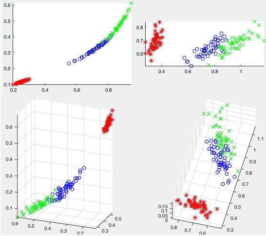
The figures above show the two datasets (the 3-D 8-class dataset at top, the 4-D 3-class iris dataset at bottom) when mapped to a 2-D space by the two methods (autoencoder on left, KLT on right). We note that the distribution of the data points are similar in the 2-D spaces resulted from the two methods, indicating these spaces are spanned by similar basis vectors, i.e., the weight vectors of the two hidden layer nodes are similar to the eigenvectors used in the KLT. However, by visual observation, the class separability in the 2-D space produced by the autoencoder (left) seems to be better than that by the KLT (right), which is also conformed quatitatively.

We Note that in the first dataset, all three dimensions are equally important for the representation of the 8 classes, i.e., the dimensionality can hardly be reduced without losing significant amount of information. In fact, the three dimensions after the KLT contain roughly the same percentage of energy: $0.37\%,\;0.33\%,\;0.30\%$, i.e., reduction of dimensionality from 3 to 2 will impose a significant challenge for the subsequent classification in the space of reduced dimensionality, which can be measured by the separability and classification error rate, as listed in the table below for both autoencoder and KLT.

We see that for both datasets, the performance of the autoencoder method (to the left of the slash symbol) is always better than that of the KLT method (to the right of slash) with higher separability and lower error rate.

$$\begin{tabular}{l\vert\vert l\vert l}\hline & Separability & Erro... ...\\ \hline \mbox{Iris Dataset} & 1.12/1.07 & 0.020/0.027 \\ \hline \end{tabular}$$ (70)

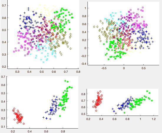
Example 2: In general, the autoencoder network is trained by all samples in the dataset. However, if all samples in a dataset are labeled to belong to one of a set of classes, the autoencoder can also be trained by these classes. Specifically in this example, the three classes in the iris dataset each represented by the average of all samples in the class are used to train the autoencoder. The figure below shows the 4-D iris dataset mapped to 2-D (top) and 3-D (bottom) spaces by both the autoencoder (left) and KLT (right). It is interesting to observe that in the case of autoencoder (left), the data points representing the three classes are arranged into a line structure in both 2 and 3-D spaces.

To encourage sparsity of the hidden layer, most of the hidden layer nodes to be inactive, we include an extra penalty term in the objective function to discourange hidden layer nodes from being activated.

There are two typical ways to do so:

• L1 or L2 regularization

  $$J=\varepsilon+\lambda\sum_{j=1}^l \vert a_j\vert,\;\;\;\;\;\; J=\varepsilon+\frac{\lambda}{2}\sum_{j=1}^l a_j^2$$ (71)

• KL-divergnece

  We first define the sparsity parameter $\rho$ for the average actiation of a hidden layer node, typically a small value close to zero (e.g., $\rho=0.05$), and also find for the jth hidden layer node its average activation over all inputs from the input layer:

  $$\hat\rho_j=\frac{1}{d}\sum_{k=1}^d z_j(x_k) =\frac{1}{d}\sum_{k=1}^d \sum_{k=1}^ ,\;\;\;\;\;\;(j=1,\cdots,l)$$ (72)

  where $z_j(x_k)$ represents how much the jth hidden layer node is affected by the kth input $x_k$. The difference between the desired sparsity in terms of $\rho$ and the actual activation $\hat\rho$ can be measured by the KL-divergence

  $$KL(\rho\vert\vert\hat\rho_j)=\rho\log\left(\frac{\rho}{\hat\rho_j}\right) +(1-\rho)\log\left(\frac{(1-\rho)}{(1-\hat\rho_j)}\right)$$ (73)

  where $\rho$ is treated as the desired probability of $x=1$ for a binary random variable (Bernoulli distribution, with probability $1-\rho$ for $x=0$), and $\hat\rho_j$ treated as the actual probability of the binary random variable. This KL-divergence is minimized when $\hat\rho=\rho$. The penalty term is the sum of the KL-divergences of all $l$ hidden layer nodes:

  $$\sum_{j=1}^l KL(\rho\vert\vert\hat\rho_j)$$ (74)

$$J({\bf W}^h,{\bf W}^o)=\varepsilon+\lambda\sum_{j=1}^l KL(\rho\vert\vert\hat\rho_j)$$ (75)

Autoencoder and PCA are similar for XOR and cocentric datasets. but different for data of digits from 0 to 9