Back Propagation

The back propagation network (BP network or BPN) is a supervised laerning algorithm that finds a wide variety of applications in practice. In the most general sense, a BPN can be used as an associator to learn the relationship between two sets of patterns represented in vector forms. Specifically in classification, similar to the perceptron network, the BPN as a classifier is based on the training set ${\bf X}=[{\bf x}_1,\cdots,{\bf x}_N]$, of which each pattern ${\bf x}_n$, a d-dimensional vector, is associated with the corresponding pattern, an m-dimensional vector ${\bf y}_n$ in ${\bf Y}=[{\bf y}_1,\cdots,{\bf y}_N]$, as its class identity labeling, indicating to to which of the $K$ classs $\{C_1,\cdots,C_K\}$ pattern ${\bf x}_i$ belongs.

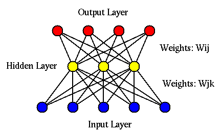
Different from the perceptron in which there is only one level of learning taking place between the output and input layers in terms of the weights, a BPN is a multi-layer (three or more) hierarchical structure composed of the input, hidden, and output layers, in which learning takes place in multilevels between consecutive layers. Consequently, a BPN can be more flexible and powerful than the two-layer perceptron network. In the following, before we consider the general BPN containg multiple hidden layers, we will first derive the back propagation algorithm for the simplest BPN with only one hidden layer in between the input and output layers.

We assume the input, hidden and output layers contain respectively $d$, $l$, and $m$ nodes, each node in the hidden and output layers is fully connected to all nodes in the previous layer. When one of the $N$ training patterns ${\bf x}$ is presented to the input layer of the BPN, an m-D vector $\hat{\bf y}=f({\bf x},{\bf W}^h,{\bf W}^o)$ is produced at the output layer as the corresponding response to the input ${\bf x}$. Here ${\bf W}^h=[{\bf w}^h_1,\cdots,{\bf w}^h_l]$ and ${\bf W}^o=[{\bf w}^o_1,\cdots,{\bf w}^o_m]$ are the function parameters containing the augmented weight vectors for both the hidden and output layers, to be determined in the training process based on the training set ${\bf X}$ and ${\bf Y}$ so that its output $\hat{\bf y}_n$ as a function of the current input ${\bf x}_n$ matches the desired output, the labeling ${\bf y}_n$. Once the BPN is fully trained, any unlabeled pattern ${\bf x}$ can then be classified into one of the $K$ classes corresponding to the minimum $\delta=\vert\vert{\bf y}-\hat{\bf y}\vert\vert$. Note that different from the perceptron network, the output of the $m$ output nodes are in general not binary, although they can still be binary if either one-hot or binary encoding is used for class labeling.

Specifically, the training of the BPN is an iteration of the following two-phase process:

• The feedforward pass:

  A randomly selected sample ${\bf x}_n$ labeled by ${\bf y}_n$ is presented to the input layer and forwarded through the weighted connections to the hidden layer and then the output layer to produce output $\hat{\bf y}=f({\bf x},{\bf W}^h,{\bf W}^o)$.

• The backward error backpropagation:

  The squared error $\varepsilon=\vert\vert{\bf y}_n-\hat{\bf y}_n\vert\vert^2/2$ measuring the difference between the desired output ${\bf y}_n$ and the actual output $\hat{\bf y}_n$ is propagated backward from the output layer through the hidden layer to the input layer, during which the weights of both the output and hidden layers are modified so that $\varepsilon$ will be reduced when the same or similar pattern is presented in the future.

This two-phase process is iteratively carried out untill eventually the error is minimized for all training samples and BPN is properly trained.

We now consider the specific computation taking place in both the forward and backward passes.

• The forward pass from input ${\bf x}=[x_1,\cdots,x_d]^T$ represented to the input layer to the output $\hat{\bf y}_n=[y_1,\cdots,y_m]^T$ produced by the output layer:
  • From input layer to hidden layer:

    $$z_j=g(a^h_j)=g\left(\sum_{k=1}^d w_{jk}^h x_k+b_j^h\right) =g\lef... ..._{k=0}^d w_{jk}^h x_k\right)=g({\bf x}^T{\bf w}^h_j) \;\;\;\;\;\;(j=1,\cdots,l)$$ (46)

    where both ${\bf x}=[x_0=1,x_1,\cdots,x_d]^T$ and ${\bf w}_j^h=[w_{j0}^h=b_j^h,w_{j1}^h,\cdots,w_{jd}^h]^T$ are augmented, and $a^h_j={\bf x}^T{\bf w}^h_j$ is the activation of the jth hidden layer node. These $l$ equations can be expressed in vector form:

    $${\bf z}={\bf g}\left({\bf W}^h{\bf x}\right)$$ (47)

    where ${\bf z}=[z_1,\cdots,z_l]^T$, and ${\bf W}^h=[{\bf w}^h_1,\cdots,{\bf w}^h_l]^T$ is an $l\times(d+1)$ matrix.

  • From hidden layer to output layer:

    $$\hat{y}_i=g(a_i^o)=g\left(\sum_{j=1}^l w_{ij}^o z_j+b_i^o\right) ... ..._{j=0}^l w_{ij}^o z_j\right)=g({\bf z}^T{\bf w}^o_i) \;\;\;\;\;\;(i=1,\cdots,m)$$ (48)

    where both ${\bf z}=[z_0=1,z_1,\cdots,z_l]^T$ and ${\bf w}_i^o=[w_{i0}^o=b_i^o,w_{i1}^o,\cdots,w_{il}^o]^T$ are augmented, and $a^o_i={\bf z}^T{\bf w}^o_i$ is the activation of the ith output layer node. These $m$ equations can be expressed in vector form:

    $$\hat{\bf y}={\bf g}\left( {\bf W}^o{\bf z} \right)$$ (49)

    where $\hat{\bf y}=[\hat{y}_1,\cdots,y_m]^T$, and ${\bf W}^o=[{\bf w}^o_1,\cdots,{\bf w}^o_m]^T$ is an $m\times(l+1)$ matrix.

• The backward error propagation from error $\varepsilon$ to the input layer:

  The squared error $\varepsilon=\vert\vert{\bf y}-\hat{\bf y}\vert\vert^2/2$ can be written as a function of the output weights $w_{ij}^o\;(i=1,\cdots,m,\;j=0,1,\cdots,l)$ and hidden layer weights $w_{jk}^h\;(j=1,\cdots,l,\;k=0,1,\cdots,d)$:
  

  $$\varepsilon = \frac{1}{2}\vert\vert{\bf y}-\hat{\bf y}\vert\vert^2 =\frac{1}{2}... ...rac{1}{2}\sum_{i=1}^m\left[g\left(\sum_{j=0}^lw_{ij}^{o}z_j\right)-y_i\right]^2$$

  $$= \frac{1}{2}\sum_{i=1}^m\left[g\left(w_{i0}^o+\sum_{j=1}^l w_{ij}^... ...m_{j=1}^l w_{ij}^o\, g\left(\sum_{k=0}^d w_{jk}^hx_k\right)\right)-y_i\right]^2$$ (50)

  
  

  Similar to the objective function of the ridge regression considered in a previous section, an additional regularization term can be included in the objective function to encourage small weights to prevent overfitting:

  $$J({\bf W}^h,{\bf W}^o)=\varepsilon +\frac{\lambda}{2}\left[\vert\vert{\bf W}^h\vert\vert _2^2+\vert\vert{\bf W}^o\vert\vert _2^2\right]$$ (51)

  where $\lambda$ is the weight decay parameter and $\vert\vert{\bf W}\vert\vert _2=\sqrt{\sum_i\sum_j w_{ij}^2}$ is the Frobenius norm.

  The gradient descent method is used to modify first the output layer weights and then the hidden layer weights to iteratively reduce the objective function $J$ in the following steps:

  • Find the gradient of $J$ with respect to the output layer weights $w_{ij}^{o}\;\;(i=1,\cdots,m,\;j=0,1,\cdots,l)$ by the chain rule:

    $$\frac{\partial\,J}{\partial\, w_{ij}^o} =\frac{\partial\,\varepsi... ...i)\;g'(a^o_i)\;z_j+\lambda w_{ij}^o =-\delta_i\;g'(a^o_i)\;z_j+\lambda w_{ij}^o$$ (52)

    where $\delta_i=y_i-\hat{y}_i$.

  • Update $w_{ij}^o\;(i=1,\cdots,m,\;j=0,1,\cdots,l)$ to reduce $J$ by gradient descent method with learning rate or step size $\eta$:
    

    $$w_{ij}^o \Leftarrow w_{ij}^o -\eta\frac{\partial J}{\partial w_{ij}^o} =w_{ij}^o -\eta \left(-\delta_i\;g'(a^o_i)\;z_j+\lambda w_{ij}^o\right)$$

    $$= w_{ij}^o-\eta\left(-d_i^o\;z_j+\lambda w_{ij}^o\right)$$ (53)

    
    where $d_i^o=\delta_ig'(a^o_i)$, or in matrix form:

    $${\bf W}^o \Leftarrow {\bf W}^o -\eta\left(-{\bf d}^o{\bf z}^T+\lambda {\bf W}^o\right) ={\bf W}^o+\eta{\bf d}^o{\bf z}^T-\eta\lambda {\bf W}^o$$ (54)

    where ${\bf d}^o=[d_1^o,\cdots,d_m^o]^T$ is the elementwise (Hadamard) product ${\bf\delta} \odot {\bf g}'({\bf a}^o)$, and ${\bf d}^o{\bf z}^T={\bf d}^o \otimes {\bf z}$ is the outer product of ${\bf d}^o$ and ${\bf z}=[z_0=1,z_1,\cdots,z_l]$.

  • Find the gradient of $J$ with respect to the hidden layer weights $w_{jk}^h\;\;(j=1,\cdots,l,\;k=0,1,\cdots,d)$ by the chain rule:

    
    

    $$\frac{\partial\,J}{\partial\, w_{jk}^h} = \frac{\partial\,\varepsilon}{\partial\, \hat{y}_i}\; \frac{\parti... ...artial\, a^h_j}\; \frac{\partial\, a^h_j}{\partial\, w_{jk}^h}+\lambda w^h_{jk}$$

    $$= -\sum_{i=1}^m \delta_ig'(a^o_i)w_{ij}^o\;g'(a^h_j)x_k +\lambda w^h_{jk} =-\left(\sum_{i=1}^m d_i^o w_{ij}^o\right) g'(a^h_j)x_k +\lambda w^h_{jk}$$

    $$= -\delta_j^{h}\;g'(a^h_j)x_k +\lambda w^h_{jk} =-d_j^h x_k +\lambda w^h_{jk}$$ (55)

    
    where we have defined

    $$\delta_j^h=\sum_{i=1}^m d_i^o w_{ij}^o,\;\;\;\;\; d^h_j=\delta^h_... ...ft(\sum_{i=1}^m d_i^o w_{ij}^o\right) g'(a_j^h), \;\;\;\;\;\;\;\;(j=1,\cdots,l)$$ (56)

    or in matrix form:

    $$\left[\begin{array}{l}\delta_1^h\\ \vdots\\ \delta_l^h\end{array}... ... \left[\begin{array}{c}d_1\\ \vdots\\ d_m\end{array}\right] ={\bf W}^o{\bf d}^o$$ (57)

    Here ${\bf W}^o$ is an $m\times l$ matrix, the same as that defined above but with the first column of $b_j$'s removed.

  • Update $w_{jk}^h\;\;(j=1,\cdots,l,\;k=0,1,\cdots,d)$ to reduce $J$ by gradient descent method:
    

    $$w_{jk}^h \Leftarrow w_{jk}^h-\eta \frac{\partial J}{\partial w_{jk}^h} =w_{jk}^h-\eta\left(-\delta_j^h\;g'(a^h_j)x_k+\lambda w_{jk}^h\right)$$

    $$= w_{jk}^h-\eta\left(-d_j^hx_k+\lambda w_{jk}^h\right)$$ (58)

    
    or in matrix form:

    $${\bf W}^h \Leftarrow {\bf W}^h -\eta\left( -{\bf W}^o{\bf d}^o \o... ...\lambda{\bf W}^h\right) ={\bf W}^h+\eta{\bf d}^h {\bf x}^T-\eta\lambda{\bf W}^h$$ (59)

    where ${\bf d}^h={\bf W}^o{\bf d}^o \odot {\bf g}'({\bf a}^h)$ is the elementwise product of vector ${\bf W}^o{\bf d}^o$ and ${\bf g}'({\bf a}^h)$, and ${\bf d}^h{\bf x}^T={\bf d}^h\otimes{\bf x}$ is the outer product of vectors ${\bf d}^h$ and ${\bf x}$.

In summary, here are the steps in each iteration:

1. Input a randomly selected pattern $[x_1,\cdots,x_d]^T$, construct $d+1$ dimensional vector ${\bf x}=[1,x_1,\cdots,x_d]^T$;

2. Compute ${\bf z}={\bf g}({\bf W}^h{\bf x})$, and construct $l+1$ dimensional vector ${\bf z} \leftarrow [1,{\bf z}]$;

3. Compute $\hat{\bf y}={\bf g}({\bf W}^o{\bf z});$

4. Get elementwise product ${\bf d}^o=({\bf y}-\hat{\bf y})\odot {\bf g}'({\bf a}^o) ={\bf\delta}\odot{\bf g}'({\bf a}^o)$;

5. Update output weights ${\bf W}^o\Leftarrow {\bf W}^o+\eta\;{\bf d}^o{\bf z}^T -\eta\lambda{\bf W}^o$;

6. Get elementwise product ${\bf d}^h={\bf W}^{oT}{\bf d}^o \odot {\bf g}'({\bf a}^h) ={\bf\delta}^h\odot {\bf g}'({\bf a}^h)$, where ${\bf W}^o_{m\times l}$ is the same as ${\bf W}^o$ but with its first column removed.

7. Update hidden weights ${\bf W}^h\Leftarrow {\bf W}^h+\eta\;{\bf d}^h{\bf x}^T -\eta\lambda{\bf W}^h$;

8. Terminate the iteration if the error $\varepsilon$ is acceptably small for all of the training patterns. Otherwise repeat the above with another pattern in the training set.

The Matlab code for the essential part of the BPN algorithm is listed below. Array $X$ contains $C$ classes each with $K$ samples, array $Y$ are the labelings of the $C*K$ training samples, array $W$ contains the $N+1$ dimensional weight vectors for the $M$ output nodes. Also, $L$ is the number of hidden nodes, $\eta$ is the learning rate between 0 and 1, and $tol$ is the tolerance for the terminination of the learning iteration (e.g., 0.01).

function [Wh, Wo, g]=backPropagate(X,Y)
    syms x 
    g=1/(1+exp(-x));              % Sigmoid activation function
    dg=diff(g);                   % its derivative function
    g=matlabFunction(g);
    dg=matlabFunction(dg);
    [d,N]=size(X);                % number of inputs and number of samples
    X=[ones(1,N); X];             % augment X by adding a row of x0=1  
    Wh=1-2*rand(L,d+1);           % Initialize hidden layer weights 
    Wo=1-2*rand(M,L+1);           % Initialize output layer weights 
    er=inf;
    while er > tol
        I=randperm(N);            % random permutation of samples
        er=0;
        for n=1:N                 % for all N samples for an epoch
            x=X(:,I(n));          % pick a training sample      
            ah=Wh*x;              % activation of hidden layer  
            z=[1; g(ah)];         % augment z by adding z0=1
            ao=Wo*z;              % activation to output layer
            yhat=g(ao);           % output of output layer 
            delta=Y(:,I(n))-yhat  % delta error
            er=er+norm(delta)/N   % test error
            do=delta.*dg(ao);     % Find d of output layer 
            Wo=Wo+eta*do*z';      % update weights for output layer 
            dh=(Wo(:,2:L+1)'*do).*dg(ah);   % delta of hidden layer 
            Wh=Wh+eta*dh*x';      % update weights for hidden layer 
        end         
    end
end

The training process of BP network can also be considered as a data modeling problem to fit the given data $\{({\bf x}_i,\,{\bf y}_i),\;(i=1,\cdots,N)\}$ by a function with the weights of both the hidden and output layers as the parameters:

$${\bf y}={\bf f}({\bf x},{\bf W}^h,{\bf W}^o)$$ (60)

The goal is to find the optimal parameters ${\bf W}^h$ and ${\bf W}^o$ that minimize the difference ${\bf r}={\bf y}-\hat{\bf y}$ between the desired and the actual outputs. The Levenberg-Marquardt algorithm discussed previously can be used to obtain the parameters, such as Matlab function trainlm.

The three-layer BPN containing a single hidden layer discussed above can be easily generalized to a multilayer BPN containing any number of hidden layers (e.g., for a deep learning network) by simply repeating steps 6 and 7 for the single hidden layer in the algorithm list above. We assume in addition to the input layer, there are in total $L$ learning layers including all the hidden layers and the output layer, indexed by $l=1,\cdots,L$. Then step 6 above becomes:

$${\bf d}^{(l)}={\bf\delta}^{(l)}\cdot{\bf g}'({\bf a}^{(l)}) \;\;\;\;\;\; (l=1,\cdots,L)$$ (61)

where ${\bf a}^{(l)}=({\bf W}^{(l)}{\bf z}^{(l)})$ is the activation of all nodes in the lth layer, ${\bf z}^{(l)}={\bf W}^{(l-1)}{\bf z}^{(l-1)}$ is the input to the lth layer, output from the (l-1)th layer ( ${\bf z}^{(1)}={\bf x}$), and

$${\bf\delta}^{(l)}=\left\{\begin{array}{ll} {\bf y}-\hat{\bf y} & (l=L)\\ {\bf W}^{(l)}{\bf d}^{(l-1)} & (1 \le l <L)\end{array}\right.$$ (62)

Then the same step 7 for updating the weights can be carried out based on the gradient vector:

$${\bf d}^{(l)} \otimes {\bf z}^{(l)} ={\bf d}^{(l)} ({\bf z}^{(l)})^T$$ (63)

The matlab code segment below is for the BP network of multiple hidden layers, in which $L$ is the total number of learning layers and $m(l)$ is the number of nodes in the lth layer ( $l=1,\cdots,L$):

    W={1-2*rand(m(1),d+1)};                 % initial weights for first layer
    for l=2:L
        W{l}=1-2*rand(m(l),m(l-1)+1);       % initial weights for all other layers
    end
    er=inf;
    while er > tol
        I=randperm(N);                      % random permutation of samples
        er=0;
        for n=1:N                           % N samples for an epoch
            z={1;X(:,I(n))};                % pick a training sample
            a={W{1}*z{1}};                  % activation of first layer
            for l=2:L                       % the forward pass
                z{l}=[1;g(a{l-1})];         % input to the lth layer 
                a{l}=W{l}*z{l};             % activation of the lth layer 
            end
            yhat=g(a{L});                   % actual output of last layer
            delta=Y(:,I(n))-yhat;           % delta error
            er=er+norm(delta)/N;            % test error
            d{L}=delta.*dg(a{L});           % d for output layer
            W{L}=W{L}+eta*d{L}*z{L}';       % upddate weights for output layer 
            for l=L-1:-1:1                  % the backward pass
                d{l}=(W{l+1}(:,2:end)'*d{l+1}).*dg(a{l});  % d for hidden layers
                W{l}=W{l}+eta*d{l}*z{l}';   % upddate  weights for hidden layers
            end  
        end
    end

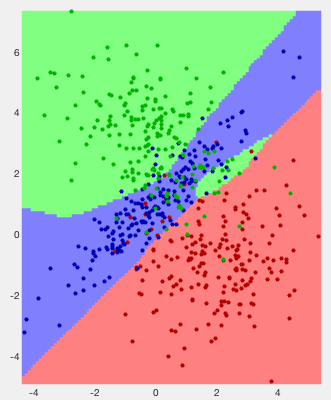
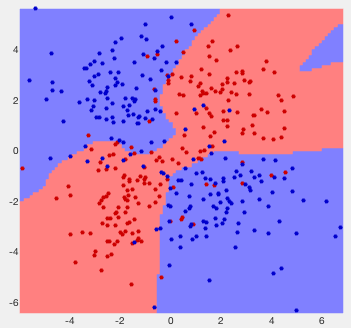
Example 1: The classification results of two previously used 2-D data sets are shown below. The error rates are respectively $13\%$ and $11.5\%$, and the confusion matrices are:

$$\left[ \begin{array}{rrr} 185 & 14 & 1 \\ 5 & 181 & 14 \\ 11 & 33... ... \;\;\;\;\;\;\; \left[ \begin{array}{rr}176 & 24 \\ 22 & 178 \end{array}\right]$$ (64)

Example 2:

The back propagation network applied to the classification of the dataset of handwritten digits from 0 to 9 used previously. Out of the $N=2240$ samples in the dataset, half is used for training while the other half for testing. Shown below are the confusion matrices of both the training (left) and testing (right) phases. Out of the 1120 samples for training 27 are misclassified ($2.4\%$), and out of the 1120 samples for testing 74 are misclassified ($6.6\%$).

$$\left[ \begin{array}{rrrrrrrrrr} 113 & 0 & 0 & 0 & 0 & 0 & 0 & 1 ... ... & 2 & 97 & 5 \\ 0 & 2 & 0 & 0 & 4 & 0 & 0 & 0 & 0 &102 \\ \end{array}\right]$$ (65)

Hierarchical structure and two pathways of the visual cortex