Karhunen-Loeve Transformation

A data point in a d-dimensional space is represented by a vector ${\bf x}=[x_1,\cdots,x_d]^T$, of which the components are the coordinates along the $d$ standard orthonomal basis vectors $\{ {\bf e}_1,\cdots,{\bf e}_d\}$ that spann the space:

$${\bf x} = \left[\begin{array}{c}x_1\\ x_2\\ \vdots\\ x_d\end{array}\right] ... ...begin{array}{c}0\\ \vdots\\ 0\\ 1\end{array}\right] =\sum_{i=1}^d x_i {\bf e}_i$$

$$= \left[\begin{array}{ccc}&&\\ {\bf e}_1&\cdots&{\bf e}_d\\ &&\end... ...ght] \left[\begin{array}{c}x_1\\ \vdots\\ x_d\end{array}\right] ={\bf I}{\bf x}$$ (44)

where ${\bf I}=[{\bf e}_1,\cdots,{\bf e}_d]$ is the identity matrix.

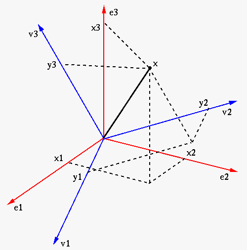
The space can also be spanned by any other orthonormal basis $\{{\bf a}_1,\cdots,{\bf a}_d\}$ satisfying

$${\bf a}_i^T{\bf a}_j=\delta_{ij}=\left\{\begin{array}{ll} 1 & i=j \\ 0 & i\ne j\end{array}\right.$$ (45)

and the same vector ${\bf x}$ can also be represented as a weighted vector sum of these basis vectors:

$${\bf x}=\sum_{i=1}^d y_i {\bf a}_i =\left[\begin{array}{ccc}&&\\ ... ...ight] \left[ \begin{array}{c} y_1\\ \vdots \\ y_d \end{array} \right] ={\bf Ay}$$ (46)

where ${\bf A}=[{\bf a}_1,\cdots,{\bf a}_d]$ composed of $d$ orthonormal column vectors is an orthogonal matrix satisfying ${\bf AA}^T={\bf A}^T{\bf A}={\bf I}$, and ${\bf y}=[y_1,\cdots,y_d]^T$ is a vector containing all $d$ coordinates in the directions of the basis vector $\{{\bf a}_i,\cdots,{\bf a}_d\}$, which can be found by premultiplying ${\bf A}^T={\bf A}^{-1}$ on both sides of the equation above ${\bf Ay}={\bf x}$:

$${\bf A}^T{\bf Ay}={\bf y} =\left[ \begin{array}{c} y_1\\ \vdots \... ...in{array}{c}{\bf a}_1^T{\bf x}\\ \vdots\\ {\bf a}_d^T{\bf x} \end{array}\right]$$ (47)

of which the ith coordinate $y_i={\bf a}_i^T{\bf x}$ is the projection of ${\bf x}$ onto the ith basis vector ${\bf a}_i$.

The basis vectors in ${\bf A}=[{\bf a}_1,\cdots,{\bf a}_d]$ can be considered as a rotated version of the standard basis in ${\bf I}=[{\bf e}_1,\cdots,{\bf e}_d]$, and the norm or length of ${\bf x}$ before and and ${\bf y}$ after the transform remain the same:

$$\vert\vert{\bf x}\vert\vert^2={\bf x}^T{\bf x}=\left(\sum_{i=1}^d... ...y_iy_j \;{\bf a}_i^T{\bf a}_j =\sum_{i=1}^d y_i^2=\vert\vert{\bf y}\vert\vert^2$$ (48)

This identity can be considered as the generalized version of Parseval's identity in the Fourier transform, as a special form of unitary transform (complex version of orthogonal transform).

Summarizing the above, we can define an orthogonal transform based on any orthogonal matrix ${\bf A}$:

$$\left\{ \begin{array}{ll} {\bf y}={\bf A}^T{\bf x} & \mbox{forward transform}\\ {\bf x}={\bf Ay} & \mbox{inverse transform}\end{array}\right.$$ (49)

by which any vector ${\bf x}$ under the implicit standard basis, the column vectors of ${\bf I}=[{\bf e}_1,\cdots,{\bf e}_d]$, is transformed into ${\bf y}={\bf A}^T{\bf x}$ under the explicit basis, the column vectors of ${\bf A}=[{\bf a}_1,\cdots,{\bf a}_d]$.

Any orthogonal transform ${\bf y}={\bf A}^T{\bf x}$ is actually a rotation of the standard basis $\{ {\bf e}_1,\cdots,{\bf e}_d\}$ into another orthonormal basis $\{{\bf a}_1,\cdots,{\bf a}_d\}$ spanning the same space, while ${\bf x}$ and ${\bf y}$ are just the coordinates or coefficients of the same vector under these two different coordinate systems.

If ${\bf x}$ is treated as a random vector, then the linear transform ${\bf y}={\bf A}^T{\bf x}$, is also a random vector, and its mean vector and covariance can be found as:

$${\bf m}_y = E[ {\bf y} ]=E[ {\bf A}^T{\bf x} ] ={\bf A}^T E[ {\bf x} ]={\bf A}^T{\bf m}_x$$

$${\bf\Sigma}_y = E[ {\bf yy}^T ]-{\bf m}_y{\bf m}_y^T =E[ {\bf A}^T{\bf x}{\bf x}^T{\bf A} ] -{\bf A}^T{\bf m}_x{\bf m}_x^T{\bf A}$$

$$= {\bf A}^T[ E[ {\bf x}{\bf x}^T ]-{\bf m}_x{\bf m}^T]{\bf A} ={\bf A}^T{\bf\Sigma}_x{\bf A}$$ (50)

In particular, the Karhunen-Loeve Transform (KLT) is just one of such orthogonal transforms in the form of ${\bf y}={\bf V}^T{\bf x}$, where the orthogonal transform matrix ${\bf V}=[{\bf v}_1,\cdots,{\bf v}_d]$ is the eigenvector matrix of the covariance matrix ${\bf\Sigma}_x$ of ${\bf x}$, composed of the $d$ normalized eigenvectors of ${\bf\Sigma}_x$. As in general the covariance matrix ${\bf\Sigma}_x$ is symmetric and positive definite, its eigenvalues $\{\lambda_1,\cdots,\lambda_d\}$ are real and positive, and its eigenvectors are orthogonal, i.e., its eigenvector matrix ${\bf V}$ is indeed an orthogonal matrix satisfying ${\bf V}^T={\bf V}^{-1}$ or ${\bf V}^T{\bf V}={\bf I}$.

The $d$ eigenvalues $\{\lambda_1,\cdots,\lambda_d\}$ and the corresponding eigenvectors $\{ {\bf v}_1,\cdots,{\bf v}_d\}$ can then be found by solving the eigenequations:

$${\bf\Sigma}_x {\bf v}_i=\lambda_i{\bf v}_i\;\;\;\;\;\;(i=1,\cdots,d)$$ (51)

which can be combined to be expressed in matrix form:

$${\bf\Sigma}_x{\bf V}={\bf\Sigma}_x[{\bf v}_1,\cdots,{\bf v}_d] =[... ...dots&\ddots&\vdots\\ 0&\cdots&\lambda_d \end{array}\right] ={\bf V}{\bf\Lambda}$$ (52)

where ${\bf\Lambda}=diag(\lambda_1, \cdots, \lambda_d)$ is a diagonal matrix. Premultiplying ${\bf V}^T={\bf V}^{-1}$ on both sides, we get

$${\bf V}^T{\bf\Sigma}_x{\bf V}={\bf V}^{-1}{\bf V}{\bf\Lambda}={\bf\Lambda}$$ (53)

Taking inverse on both sides, we also get

$$( {\bf V}^T{\bf\Sigma}_x{\bf V} )^{-1} = {\bf V}^{-1}{\bf\Sigma}_x^{-1}({\bf V}^T )^{-1} = {\bf V}^T{\bf\Sigma}_x^{-1}{\bf V}={\bf\Lambda}^{-1}$$ (54)

We see that both ${\bf\Sigma}_x$ and its inverse ${\bf\Sigma}_x^{-1}$ are diagonalized by the orthogonal eigenvector matrix ${\bf V}$ to become ${\bf\Lambda}$ and ${\bf\Lambda}^{-1}$ respectively.

Based on the orthogonal eigenvector matrix ${\bf V}$, the KLT is defined as:

$${\bf y}=\left[ \begin{array}{c} y_1\\ \vdots \\ y_d \end{array} \... ...n{array}{c} {\bf v}_1^T{\bf x}\\ \vdots\\ {\bf v}_d^T{\bf x} \end{array}\right]$$ (55)

of which the ith component $y_i={\bf v}_i^T{\bf x}$ is the projection of ${\bf x}$ onto the ith eigenvector ${\bf v}_i$. Premultiplying ${\bf V}=({\bf V}^T)^{-1}$ on both sides of the forward transform ${\bf y}={\bf V}^T{\bf x}$, we get the inverse KLT transform, by which vector ${\bf x}$ is represented as a linear combination of the eigenvectors $\{ {\bf v}_1,\cdots,{\bf v}_d\}$ as the basis vectors:

$${\bf x}={\bf V} {\bf y}=\left[\begin{array}{cccc}&&\\ {\bf v}_1&... ...n{array}{c} y_1\\ \vdots \\ y_d \end{array} \right] =\sum_{i=1}^d y_i {\bf v}_i$$ (56)

Example:

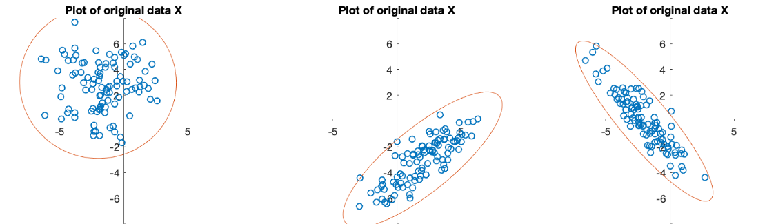
$${\bf\Sigma}_1=\left[\begin{array}{rr}2.964 & 0.544\\ 0.544 & 4.68... ...gma}_3=\left[\begin{array}{rr}3.043 & -3.076\\ -3.076 & 3.930\end{array}\right]$$ (57)

$$r_1=0.146,\;\;\;\;\;\;\;\;\;r_2=0.817,\;\;\;\;\;\;\;\;r_3=-0.889$$ (58)

$$\lambda_{1,2}=(4.845,\;2.807),\;\;\;\;\;\; \lambda_{1,2}=(7.207,\;0.659),\;\;\;\;\;\; \lambda_{1,2}=(6.594,\;0.379)$$ (59)