Competitive Learning Networks

Competitive learning is a neural network algorithm for unsupervised clustering, similar to the K-means algorithm considered previously. The competitive learning takes place in a two-layer network composed of an input layer of $d$ nodes that receives an input vector ${\bf x}=[x_1,\cdots,x_d]^T$ as a point in the d-dimensional feature space, and an output layer of $m$ nodes that produces an output pattern ${\bf y}=[y_1,\cdots,y_m]^T$ representing the clusters of interest. Each input variable $x_i$ may take either a continuous real value or a binary value depending on the specific application, the outputs $y_i\in\{0,\;1\}$ are binary, of which only one is 1 while all others are 0 (one-hot), as the result of a winner-take-all completition based on their activation values.

In each iteration of the learning process, a pattern ${\bf x}$ randomly chosen from the unlabeled dataset ${\bf X}=[{\bf x}_1,\cdots,{\bf x}_N]$ is presented to the input layer of the network, while each node of the output layer gets an activation value, a linear combination of all such $d$ inputs, i.e., the inner product of its weight vector ${\bf w}_i$ and the input vector ${\bf x}$:

$$a_i=\sum_{j=1}^d w_{ij} x_j={\bf w}_i^T{\bf x} =\vert\vert{\bf w}_i\vert\vert\;\vert\vert{\bf x}\vert\vert\;\cos\theta \;\;\;\;\;(i=1,\cdots,m)$$ (76)

where $\theta$ is the angle between vectors ${\bf w}_i$ and ${\bf x}$ in the d-dimensinal feature space. If the data vectors are optionally normalized with unit length $\vert\vert{\bf x}\vert\vert^2=1$, i.e., they are points on the unit hypersphere in the space. Optionally if the weight vectors ${\bf w}_i$ is also normalized with $\vert\vert{\bf w}_i\vert\vert=1$, then their inner product above is only affected by the angle $\theta$ between them.

The output of the network is determined by a winner-take-all competition. The node in the output layer that is maximally activated will output 1 while all others output 0:

$$y_i=\left\{ \begin{array}{ll} 1 & \mbox{if}\;\; a_i={\bf w}_i^T{\... ...{\bf x} \\ 0 & \mbox{otherwise} \end{array} \right.,\;\;\;\;\;\;(i=1,\cdots,K)$$ (77)

The inner product ${\bf w}_i^T{\bf x}$ is closely related to the Euclidean distance $d({\bf x},\,{\bf w})=\vert\vert{\bf w}_i-{\bf x}\vert\vert$:

$$d^2({\bf w}_i,{\bf x}) = \vert\vert{\bf w}_i-{\bf x}\vert\vert^2 =({\bf w}_i-{\bf x})^T({\bf w}_i-{\bf x}) ={\bf w}_i^T{\bf w}-2{\bf w}_i^T{\bf x}+{\bf x}^T{\bf x}$$

$$= \vert\vert{\bf w}_i\vert\vert^2+\vert\vert{\bf x}\vert\vert^2-2{\... ...ert^2-2\vert\vert{\bf w}_i\vert\vert\,\vert\vert{\bf x}\vert\vert\;\cos\,\theta$$ (78)

If both ${\bf x}$ and ${\bf w}_i$ are normalized, the winning node with the maximum activation $a_i={\bf w}_i^T{\bf x}$ also has the minimum Euclidean distance $\vert\vert{\bf w}_i-{\bf x}\vert\vert$ and anglular distance $\theta$. Therefore the competition above can also be expressed as the following:

$$y_i=\left\{ \begin{array}{ll} 1 & \mbox{if } \vert\vert{\bf w}_i-... ...rt\vert \\ 0 & \mbox{otherwise} \end{array} \right., \;\;\;\;\;\;(i=1,\cdots,K)$$ (79)

The only winning node that receives the highest activation gets to modify its weight vector:

$${\bf w}_i^{new}={\bf w}_i^{old}+y_i\,\eta\;({\bf x}-{\bf w}_i^{ol... ...{\bf x}& \mbox{if }y_i=1\\ {\bf w}_i^{old}& \mbox{if }y_i=0 \end{array} \right.$$ (80)

where $0<\eta<1$ is the learning rate (step size). Optionally the new weight vector can also be renormalized. For the iteration process to gradually approach a stable clustering result, the learning rate $\eta$ needs to be reduced through the iterations from its initial value (e.g., $\eta_0=0.9$) toward 0 by a certain decay factor $\alpha$ (e.g., $\alpha=0.99$). This way the learning rate decays exponentially for the learning process to gradually slow down and becomes stabalized. The decay factor $\alpha$ depends on the size of the dataset, and it may need to be determined heuristically and experimentally.

The competitive learing is illustrated in the figure above, where the modified weight vector of the winner ${\bf w}_i^{new}$ is between ${\bf x}$ and the old ${\bf w}_j^{old}$, i.e., the effect of the learning process is that the winner's weight vector which is closest to the current input pattern ${\bf x}$ is pulled even closer to it.

Here are the iterative steps in the competitive learning:

• Step 0: Normalize all data vectors ${\bf x}$, initialize randomly the weight vectors ${\bf w}$ for the output nodes (e.g., any $m$ randomly chosen samples from the dataset): ${\bf w}_1^{(0)},\;{\bf w}_2^{(0)},\cdots,{\bf w}_m^{(0)}$, set iteration index to zero $l=1$;

• Step 1: Choose randomly an input pattern ${\bf x}$ from the dataset and calculate the activation for each of the output nodes:

  $$a_i={\bf w}_i^T{\bf x}\;\;\;\;\;\;\;(i=1,\cdots,m)$$ (81)

• Step 2: find the index of the winning node $j=\argmax_i a_i$, and update its weights:

  $${\bf w}_j^{(l+1)}={\bf w}_j^{(l)} +\eta ({\bf x}-{\bf w}_i^{(l)})$$ (82)

  Reduce learning rate $\eta\leftarrow \alpha \eta$. Optionally, renormalize ${\bf w}_j^{(l+1)}$.

• Step 3: Terminate the iteration if the clustering result has gradually stablized, when the learning rate $\eta$ is reduced from its initial value $\eta_0$ to some small value (e.g., 0.1) and the weight vectors no longer change significantly. Otherwise $l \leftarrow l+1$, go back to Step 1.

This iterative process can be more intuitively understood as shown in the figure below. Every time a sample ${\bf x}$ (a red dot) is presented to the input layer, one of the output nodes will become the winner and its weight vector ${\bf w}$ (an blue x) closest to the current input ${\bf x}$ is drawn even closer to ${\bf x}$. As this process is carried out iteratively many times, each cluster of similar sample points in the space will draw one of the weight vectors towards its centeral area, and the corresponding output node will always win and output 1 whenever any member of the cluster is presented to the network in the future. In other words, after this unsupervised learning, the feature space is partitioned into $K$ regions each corresponding to one of the $K$ clusters, represented by one of the output nodes, whose weight vector is in the central area of the region. We see that this process is very similar to the K-means clustering algorithm, in which each cluster is represented by the mean vector of all of its members.

It is possible in some cases that the data samples are not distributed in such a way that they form a set of clearly saperable clusters the feature space. In the extreme case, they may even form a continuum. In such cases, a small number of output nodes (possibly even just one) may become frequent winners, while others become “dead nodes” if they never win and consequently never get the chance to odify their weight vectors. To avoid such meaningless outcome, a mechanism is needed to ensure that all nodes have some chance to win. This can be implemented by including an extra bias term in the learning rule:

$$a_i={\bf w}_i^T{\bf x}+b_i$$ (83)

where $b_i$ is the bias term proportional to the difference between the “fair share” of winning $1/m$ and the actual winning frequency:

$$b_i=c\;\left(\frac{1}{m} -\frac{\mbox{number of winnings of the ith node}} {\mbox{total number iterations so far}}\right)$$ (84)

The value of the bias term $b_i$ for the ith node will change its winning frequency. If the node is winning more than its share $1/m$, then $b_i<0$ and it becomes harder for it to win in the future. On the other hand, if the node rarely wins, $b_i>0$ and its chance to win in the future is increased. Here hyperparameter $c$ is some scaling coefficient. The greater $c$, the more balanced the competition will be. It needs to be fine tuned based on the specific nature of the data being analyzed.

This process of competitive learning can also be viewed as a vector quantization process, by which the continuous vector space is quantized to become a set of $K$ discrete regions, called Voronoi diagram (tessellation). Vector quantization can be used for data compression. A cluster of similar signals ${\bf x}$ in the vector space can all be approximately represented by the weight vector ${\bf w}$ of one of a small number of $K$ output nodes in the neighborhood of ${\bf x}$, thereby the data size can be significantly reduced.

The Matlab code for the iteration loop of the algorithm is listed below.

    [d N]=size(X);                 % dataset containing N samples
    b=zeros(1,K);                  % bias terms for K clusters
    freq=zeros(1,K);               % winning frequencies
    eta=0.9;                       % initial learning rate
    decay=0.99;                    % decay rate
    it=0;
    while eta>0.1                  % main iterations
        it=it+1;
        W0=W;                      % initial weight vectors          
        x=X(:,randi(N,1));         % randomly select an input sample
        dmin=inf;
        for k=1:K                  % find winner among all K output nodes
            d=norm(x-W(:,k))-b(k);
            if dmin>d
                dmin=d; m=k;       % mth node is the winner
            end
        end   
        w=W(:,m)+eta*(x-W(:,m));   % modify winner's weights
        W(:,m)=w/norm(w);          % renormalize its weights (optional)
        share(m)=share(m)+1;       % update share for winner
        b=c*(1/K-share/it);        % modify biases for all nodes
        eta=eta*decay;             % reduce learning rate 
    end

Examples

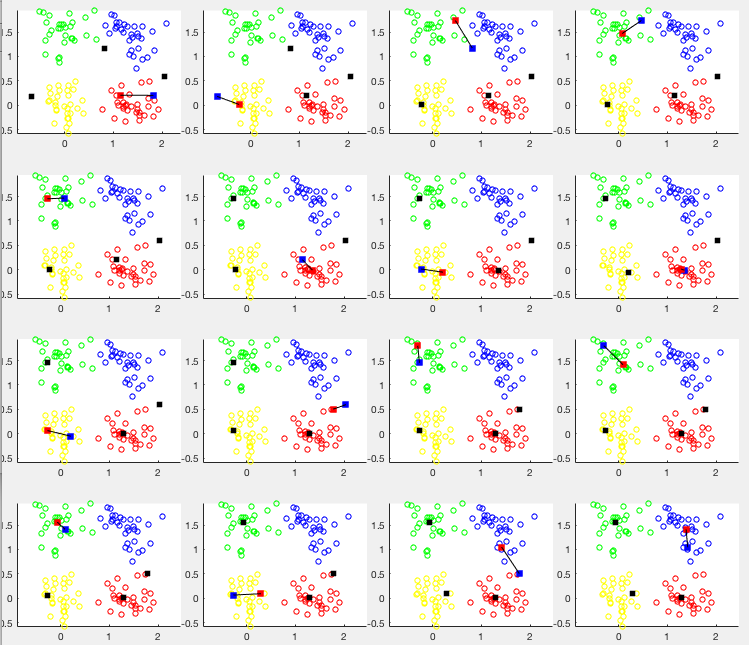
The competitive learning method is applied to a set of simulated 2-D data of four clusters. The network has $d=2$ input nodes and $K=4$ output nodes. The first 16 iterations are shown in the figure below, where open circles represent the data points, while the solid back squares represent the weight vectors. Also, the blud and red squares represent the weight vector of the winner before and after its modification, visualized by the straight line connecting the two squares. We see that the $K=4$ weight vectors randomly initialized are iteratively modified one at a time, and after these 16 iterations, they each move to the center of one of the four clusters. The saperability of the clustering result measured by $tr{\bf S}_T^{-1}{\bf S}_B$ is 1.0. When the number of output nodes is reduced to 3 and 2, the saperability is also reduced to 0.76 and 0.46, respectively. When $K=5$ output nodes are used, one of the four clusters is represented by two output nodes.

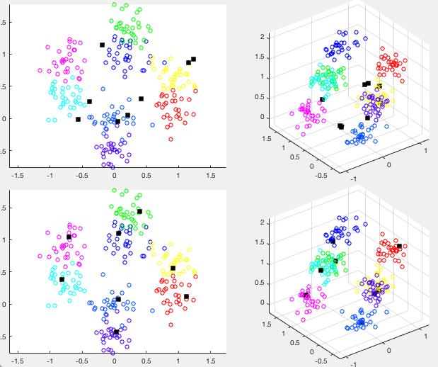
The same method is applied to a set of 3-D data of eight clusters. The results are shown in the figure below, where the top and bottom rows show the data and weight vectors before and after clustering, respectively. The left column shows the 2-D space spanned by the first two principal components, while the right column shows the original 2-D space. Again we see that the weight vectors move from their random initial locations to the centers of the eight clusters as the result of the clustering.

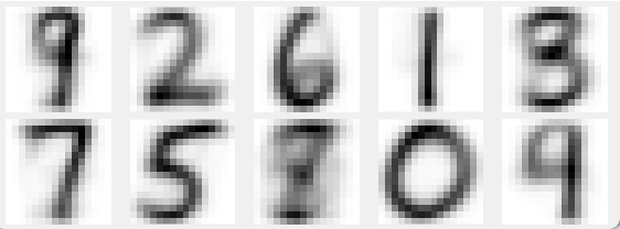
The competitive learning algorithm is also applied to the dataset of handwritten digits from 0 to 9, and the clustering result is shown as the average of all samples in each cluster in $16 \times 16$ image form shown in the figure below.