Perceptron

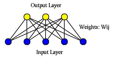
The perceptron network (F. Rosenblatt, 1957) is a two-layer learning network containing an input layer of $d$ nodes and an output layer of $m$ output node. The perceptron is a supervised method trained by dataset ${\bf X}=[{\bf x}_1,\cdots,{\bf x}_N]$, of which each sample ${\bf x}=[x_1,\cdots,x_d]^T$ is labeled by the corresponding component in ${\bf y}=[y_1,\cdots,y_N]^T$, indicating to which one of $K$ catagoric classes ${\bf x}_n$ belongs to. The goal of the training process is to determine the weights ${\bf w}=[w_1,\cdots,w_d]^T$ and bias $b$ so that the output $\hat{y}_n=\sum_{i=1}^d w_ix_n+b$ corresponding to input ${\bf x}_n$ matches its labeling $y_n$ for all $N$ samples in the training set in some optimal way. When the perceptron network is fully trained, it can be used to classify any unlabeled sample ${\bf x}$ into one of the $K$ classes.

We first consider the special case where the output layer has only $m=1$ node, and the perceptron is a binary classifier, same as the method of linear regression, and also the initial setup of the support vector machine (SVM), in the sense that all such methods are based on the linear equation $f({\bf x})={\bf w}^T{\bf x}+b=0$, representing a hyperplane by which the d-dimensional feature space is partitioned into two regions corresponding to two classes $C_+$ and $C_-$. When the parameters ${\bf w}$ and $b$ are determined in the training process, any unlabeled ${\bf x}$ is classified into either of the two classes depending on whether the function value $\hat{y}=f({\bf x})$ is greater or smaller than zero:

$$\;\; f({\bf x})={\bf w}^T{\bf x}+b \; \left\{ \begin{array}{l} > 0\\ <0 \end{array} \right., \;\;\; \;\;\; \hat{y}=\sign (f({\bf x})) =\left\{ \begin{array}{rl} 1 & \mbox{for } {\bf x}\in C_+\\ -1 & \mbox{for } {\bf x}\in C_-\end{array} \right.$$ (29)

If we divide the equation $f({\bf x})={\bf w}^T{\bf x}+b=0$ by $\vert\vert{\bf w}\vert\vert$, we get

$$p_{\bf w}({\bf x})=\frac{{\bf w}^T{\bf x}}{\vert\vert{\bf w}\vert\vert} =-\frac{b}{\vert\vert{\bf w}\vert\vert}=b'$$ (30)

where $p_{\bf w}({\bf x})={\bf w}^T{\bf x}/\vert\vert{\bf w}\vert\vert$ is the projection of ${\bf x}$ onto the normal direction ${\bf w}$ of the partitioning hyperplane, and $b'=-b/\vert\vert{\bf w}\vert\vert$ is the vector from the origin to the hyperplane ($\vert b'\vert$ is the distance of the hyperplane to the origin). Now the classification above can be rewritten as

$$\;\; p_{\bf w}({\bf x}) \left\{ \begin{array}{l} > b'\\ <b' \end{array} \right., \;\;\; \;\;\; {\bf x}\in\left\{ \begin{array}{l}C_+\\ C_-\end{array}\right.$$ (31)

We see that in all binary classification methods, an unlabeled sample ${\bf x}$ is classified into either of the two classes based on the projection $p_{\bf w}({\bf x})$ of ${\bf x}$ onto ${\bf w}$, which is either greater or smaller than the bias $b'$, depending on whether ${\bf x}$ is on the positive or negative side of the plane.

In all these binary classification methods the parameters ${\bf w}$ and $b$ need to be determined based on training set ${\bf X}$ labeled by ${\bf y}$, but they do so differently. While in least squares method and support vector machine these parameters are obtained by respectively the least squared method and quadratic programming, here in the perceptron network these parameters are obtained by iteratively modifying some randomly initialized values to gradually reduce the error or residual, the difference between actual output $\hat{y}_n=f({\bf x}_n)$ and the ground truth labeling $y_n$, denoted by $\delta=y_n-\hat{y}_n$, for all training samples in the dataset. This method is called the $\delta$-rule.

We now consider specifically the training algorithm of the perceptron network as a binary classifier. As always, we redefine the data vector as ${\bf x}=[x_0=1,x_1,\cdots,x_n]^T$ and the weight vector as ${\bf w}=[w_0=b,w_1,\cdots,w_n]^T$ so that the decision function can be more conveniently written as an inner product $f({\bf x})={\bf w}^T{\bf x}$ without the additional bias term.

The randomly initialized weight vector ${\bf w}$ is iteratively updated based on the following mistake driven $\delta$-rule:

$${\bf w}^{new}={\bf w}^{old}+\eta(y-\hat{y})\,{\bf x} ={\bf w}^{old}+\eta\,\delta{\bf x}$$ (32)

where $\eta>0$ is the step size but here called the learning rate, which is assumed to be 1 in the following for simplicity. We can show that by the iteration above, ${\bf w}$ is modified in such a way that the error $\delta$ is always reduced.

When a training sample ${\bf x}$ labeled by $y\pm 1$ is presented to the nodes of the input layer of the perceptron, its output $\hat{y}=\sign (f({\bf x}))$ may or may not match the the label $y$, as shown in the table:

$$\begin{tabular}{c\vert l\vert l\vert l} \hline & $y$\ & $f({\bf x... ... & $y=-1$\ & $f({\bf x})<0,\;\hat{y}=-1$\ & $\delta=0$\ \\ \hline \end{tabular}$$ (33)

In both the first and last cases, $y f({\bf x})>0$, the error is $\delta=y-\hat{y}=0$, and the weight vector ${\bf w}^{new}={\bf w}^{old}+\delta{\bf x}={\bf w}^{old}$ is not modified. But in cases 2 and 3 $y f({\bf x})<0$, the error is $\delta=y-\hat{y}=1$, the weight vector ${\bf w}$ is modified in either of the following two ways:

• In case 2, $y=-1$, but $\hat{y}=1$, then $y\,f({\bf x})<0$ and $\delta=-2$, we have

  $${\bf w}^{new}={\bf w}^{old}-2{\bf x}$$ (34)

  When the same ${\bf x}$ is presented to the network again in the future, the function is smaller than its previous value

  $$f({\bf x})={\bf x}^T{\bf w}^{new} ={\bf x}^T{\bf w}^{old}-2{\bf x}^T{\bf x} < {\bf x}^T{\bf w}^{old}$$ (35)

  and the output $\hat{y}$ is more likely to be the same as the desired $y=-1$.

• In case 3, $y=1$, but $\hat{y}=-1$, then $y\,f({\bf x})<0$ and $\delta=2$, we have

  $${\bf w}^{new}={\bf w}^{old}+2{\bf x}$$ (36)

  When the same ${\bf x}$ is presented again, the function is greater than its previoius value

  $$f({\bf x})={\bf x}^T{\bf w}^{new} ={\bf x}^T{\bf x}^{old}+2{\bf x}^T{\bf x} > {\bf x}^T{\bf w}^{old}$$ (37)

  and the output $\hat{y}$ is more likely to be the same as the desired $y=1$.

The update equations in Eq. (34) for $y=-1$ and Eq. (36) for $y=-1$ can be combined to become

$${\bf w}^{new}={\bf w}^{old}+y {\bf x}$$ (38)

where the scaling constant $2$ is dropped as it can be absorbed into the learning rate if we let $\eta=1/2$. Now the learning rule can be rewritten as:

$$\;\;\;\;y\,f({\bf x})\left\{\begin{array}{c} >0\\ <0 \end{array}\right. \;\;\; \;\;\;\;\; \left\{\begin{array}{l} {\bf w}^{new}={\bf w}^{old} \\ {\bf w}^{new}={\bf w}^{old}+y\,{\bf x} \end{array}\right.$$ (39)

In summary, the learning law guarantees that the weight vector ${\bf w}$ is modified in such way that the performance of the network is always improved with reduced error $\delta=y-\hat{y}$. If $C_+$ and $C_-$ are linearly saperable, then a perceptron will always produce ${\bf w}$ in finite number of iterations to saperate them.

This binary classifier with $m=1$ output node can now be genrealized to multiclass classifier with $m>1$ output nodes, and each of the $m$ weight vectors in ${\bf W}=[{\bf w}_1,\cdots,{\bf w}_m]$ is modified by the same learning process considered above. The $K>2$ classes can be encoded by the $m$ outputs $y_i\in\{-1,\,1\},\;(i=1,\cdots,m)$ in two different ways. If the one-hot method is used, the $m$ binary output can encode $K=m$ classes, i.e., the kth class is represented by an m-bit output with $y_k=1$ while all others $y_l=-1$ for $l\ne k$. Alternatively, if binary encoding is used, the $m$ outputs can encode as many as $K=2^m$ classes. For example, $K=4$ classes can be labeled by $4$ binary vector of either 4 or 2 bits:

$$\begin{tabular}{c\vert\vert r\vert r\vert r\vert r} \hline \mbox{... ... 1 & -1 \\ \hline $y_4$\ & -1 & -1 & -1 & 1 \\ \hline \end{tabular}\;\;\;\;\;\; \;\;\;\;\;\;\; \begin{tabular}{l\vert\vert r\vert r\vert r\vert r... ...$\ & -1 & -1 & 1 & 1 \\ \hline $y_2$\ & -1 & 1 & -1 & 1 \\ \hline \end{tabular}$$ (40)

The outputs of the $m$ output nodes form an m-dimensional binary vector $\hat{\bf y}=[\hat{y}_1,\cdots,\hat{y}_m]^T$, which is to be compared with the labeling ${\bf y}$ of the current input ${\bf x}$ with error $\delta=\vert\vert{\bf y}-\hat{\bf y}\vert\vert$. When the training is complete, an unlabeled input ${\bf x}$ is classified to one of the $K$ classes with a matching label to the perceptron's output. In the case of one-hot encoding, it is possible for the binary output ${\bf y}$ to not match any of the $K$ one-hot encoded classes (e.g., $\hat{\bf y}=[-1\;1\;-1\;1]^T$. In this case, the input ${\bf x}$ can be classified to the class corresponding to the node with the greatest output value $f({\bf x})={\bf w}^T{\bf x}$.

The Matlab code for the essential part of the algorithm is listed below. Array ${\bf X}$ is the dataset contains $N$ training samples, each labeled by one of the components in array ${\bf y}$ as its class identity. Array ${\bf W}$ is a $(d+1)\times m$ matrix containing $d+1$ dimensional weight vectors each for one of the $m$ output nodes.

    [X Y]=DataOneHot;           % get data
    K=length(unique(Y','rows')) % number of classes
    X=[ones(1,N); X];           % data augmentation
    [d N]=size(X);              % number of dimensions and number of samples
    m=size(Y,1);                % number of output nodes
    W=2*rand(d,m)-1;            % random initialization of weights
    eta=1;
    nt=10^4;                    % maximum number of iteration
    for it=1:nt       
        n=randi([1 N]);         % random index
        x=X(:,n);               % pick a training sample x
        y=Y(:,n);               % label of x
        yhat=sign(W'*x);        % binary output
        delta=y-yhat;           % error between desired and actual outputs
        for i=1:m
            W(:,i)=W(:,i)+eta*delta(i)*x;   % update weights for all K output nodes
        end
        if ~mod(it,N)           % test for every epoch
            er=test(X,Y,W);
            if er<10^(-9)
                break
            end
        end
        
    end

This is the function that test the training set based on estimated weight vectors in ${\bf W}$:

function er=test(X,Y,W)          % test based on estimated W, 
    [d N]=size(X);
    Ne=0;                        % number of misclassifications
    for n=1:N
        x=X(:,n);
        yhat=sign(W'*x);
        delta=Y(:,n)-yhat;
        if any(delta)            % if misclassification occurs to some output nodes
            Ne=Ne+1;             % update number of misclassifications
        end
    end
    er=Ne/N;                     % error percentage
end

This is the code that generates the training set labeled by either one-hot or binary encoding method:

function [X,Y]=DataOneHot
    d=3;
    K=8;
    onehot=1;           % onehot=0 for binary encoding
    Means=[ -1 -1 -1 -1 1 1 1 1;
        -1 -1 1 1 -1 -1 1 1;
        -1 1 -1 1 -1 1 -1 1];
    Nk=50*ones(1,K);
    N=sum(Nk);          % total number of samples
    X=[];
    Y=[];
    s=0.4;
    s=0.2;
    for k=1:K           % for each of the K classes
        Xk=Means(:,k)+s*randn(d,Nk(k));
        if onehot
            Yk=-ones(K,Nk(k)); 
            Yk(k,:)=1;        
        else            % binary encoding
            dy=ceil(log2(K));
            y=2*de2bi(k-1,dy)-1;
            Yk=repmat(y',1,Nk(k));
         end
        X=[X Xk];
        Y=[Y Yk];
    end
    Visualize(X,Y)        
end

Examples

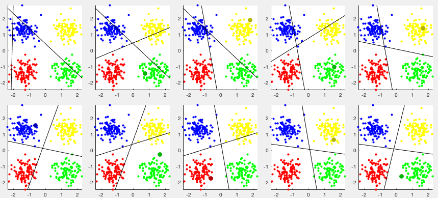
The figure below shows the classification results of a perceptron network with $n=2$ input nodes and $m=2$ output nodes. The two output nodes encode $2^2=4$ classes in a 2-D space. The training set contains 100 samples for each of the four classes labeled by ${\bf y}=[y_1,\,y_2]$. The two weight vectors ${\bf w}_1$ and ${\bf w}_2$ are initialized randomly. During the training iteration, when $\delta=y-\hat{y}\ne 0$, the weight vector for the output node is modified, otherwise, nothing needs to be done. After nine such modifications, the four classes are completely saperated by the two straight lines normal to the two weight vectors. The first panel shows the initial stage, while the subsequent panels show how the weight vectors are modified each time when $\delta\ne 0$. The darker and bigger dots represent the samples presented to the network when one of the weight vectors is modified.

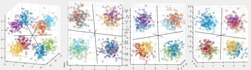
The figure below shows the classification results of a perceptron of $n=3$ input nodes and $m=3$ output nodes encoding $2^3=8$ classes. After 35 modifications the weight vectors, the perceptron is completely trained to classify all eight classes correctly. The first panel shows the initial stage, the following three panels show the weight vectors, ${\bf w}_1$, ${\bf w}_2$ and ${\bf w}_3$, also the normal vectors of the decision planes, from some three different viewing angles. We see that the eight classes are indeed saperated by the three planes normal to the weight vectors.

The main contraint of the perceptron algorithm as a binary classifier that the two classes are linearly separable can be removed by the kernel method, once the algorithm is modified in such a way that all data samples appear in the form of an inner product. Consider first the training process in which the $N$ training samples are repeatedly presented to the network, and the weight vector is modified to become ${\bf w}^{new}={\bf w}^{old}+y_n{\bf x}_n$ whenever a sample ${\bf x}_n$ labeled by $y_n$ is misclassified with $\delta=y_n-\hat{y}_n\ne 0$. If the weight vector is initialized to zero ${\bf w}=0$, then the weight vector by the updating rule in Eq. (38) can be written as a linear combination of the $N$ training samples:

$${\bf w}=\sum_{n=1}^N \alpha_n y_n {\bf x}_n$$ (41)

where $\alpha_n$ is the number of times sample ${\bf x}_n$ labeled by $y_n$ is misclassified. Upon receiving a new training sample ${\bf x}_l$ labeled by $y_l$, we have

$$f({\bf x}_l)= {\bf w}^T{\bf x}_l=\sum_{n=1}^N \alpha_n y_n {\bf x}_n^T{\bf x}_l, \;\;\;\;\;\; \;\;\;\;\;\; \hat{y}_l=\sign (f({\bf x}_l))$$ (42)

and the weight vector ${\bf w}$ is updated by the delta-rule:

$$\;\;\delta=y_l-\hat{y}_l \ne 0$$ If

$${\bf w}^{new}={\bf w}^{old}+ y_l\, {\bf x}_l =\sum_{n=1}^N \alpha_n y_n {\bf x}_n+ y_l\, {\bf x}_l$$ then

$$\;\;\; \;\;\; \alpha_l^{new}=\alpha_l^{old}+1$$ (43)

We see that only $\{\alpha_1,\cdots,\alpha_N\}$ need to be updated during the training process, while the weight vector ${\bf w}$ in Eq. (41) no longer needs to be explicitly calculated. Once the training process is complete, any unlabeled ${\bf x}$ can be classified into either of the two classes based on $\{\alpha_1,\cdots,\alpha_N\}$:

$$\;\;\; {\bf w}^T{\bf x} =\sum_{n=1}^N \alpha_n y_n {\bf x}_n^T{\bf x} \left\{\begin{array}{l} >0\\ <0\end{array}\right., \;\;\;\;\; \;\;\;\;\; {\bf x}\in\left\{\begin{array}{l}C_-\\ C_+\end{array}\right.$$ (44)

As all data samples appear in the form of inner product in both the training and testing phase, the kernel method can be applied to replace the inner product ${\bf x}_n^T{\bf x}_m$ by a kernel function $k({\bf x}_n,{\bf x}_m)$. Also, the discussion above for $m=1$ output nodes can be generalized to $m>1$ output nodes.

Here is the Matlab code segment for the most essential parts of the kernel perceptron algorithm:

    [X Y]=Data;                     % get dataset
    [d N]=size(X);                  % d: dimension, N: number of training samples
    X=[ones(1,N); X];               % augmented data
    m=size(Y,1);                    % number of output nodes
    A=zeros(m,N);                   % initialize alpha for all m output nodes and N samples
    K=Kernel(X,X);                  % get kernel matrix of all N samples
    for it=1:nt                     
        n=randi([1 N]);             % random index
        x=X(:,n);                   % pick a training sample     
        y=Y(:,n);                   % and its label
        yhat=sign((A.*Y)*K(:,n));   % get yhat
        delta=Y(:,n)-yhat;     	    % error between desired and actual output
        for i=1:m                   % for each output node
           if delta(i)~=0           % if a misclassification
               A(i,n)=A(i,n)+1;     % update the corresponding alpha
           end
        end    
        if ~mod(it,N)               % test for every epoch
            er=test(X,Y,A);         % percentage of misclassification
            if er<10^(-9)           
                break
            end
        end
    end

function er=test(X,Y,A)             % function for testing
    [d N]=size(X);                  % d: dimension, N: number of training samples
    m=size(Y,1);
    Ne=0;                           % initialize number of misclassifications
    for n=1:N                       % for all N training samples
        x=X(:,n);                   % get the nth sample
        y=Y(:,n);                   % and its label
        f=(A.*Y)*Kernel(X,x);       % f(x)
        yhat=sign(f);               % yhat=sign(f(x))
        if norm(y-yhat)~=0          % misclassification at some output nodes 
            Ne=Ne+1;                % increase number of misclassification
        end
    end
    er=Ne/N;                        % percentage of misclassification
end

Example:

The kernel perceptron is applied to the dataset of handwritten digits of $K=10$ classes for the digits from 0 to 9 with $m=10$ one-hot output nodes, based on the radial basis kernel. The kernel perceptron is trained on half of the data and then tested by the other half of the data. The confussion matricies of the training set by the end of the training process and the test set are both shown below. The error rate of the training set is zeor, i.e., all training samples are correctly classified, while the test error rate is $0.11$, i.e., $89\%$ of the test samples are correctly classified.

$$\left[\begin{array}{rrrrrrrrrr} 116 & 0 & 0 & 0 & 0 & 0 & 0 & 0 &... ... 1 & 3 & 93 & 4\\ 1 & 2 & 0 & 1 & 7 & 0 & 0 & 3 & 6 & 96\\ \end{array}\right]$$ (45)

The constraint of the perceptron algorithm is the requirement that the classes are linear saperabe due to the fact that there is only one level of learning taking place between the output and input layers. This constraint of linear separablity will be removed when multi-layer networks are used, such as the back propagation algorithm to be discussed in the next section, and more generally, the deep learning networks containing a large number of learning layers between the input and output layers.