- Constant gain

 |
(499) |
- Delay factor:

 |
(500) |
- Derivative factor
 :
:
 |
(501) |
In particular:
Also consider two additional cases related to  . First,

 |
(503) |
The slop of the Lm plot is
 . For example, when
  , we have:
 |
(504) |
Second, the plots of
 are similar to those of
  , except the
zero-crossing occurs at
 , i.e.,
 .
.
- Integral factor
 :
:
 |
(505) |
The Lm plot of  is a straight line with a slop of -20 dB/dec that goes
through a zero-crossing at
  .
.
- First order factor in numerator

 |
(506) |
 |
(507) |
 |
(508) |
Consider the following three cases:
The straight-line asymptote of
 has zero slope when
 but a slope 20 dB/dec when
 . The straight-line asymptote of
 is zero when
 ,
,  when
when
 ,
but with a slope
 in between.
- First order factor in denominator

 |
(512) |
 |
(513) |
Both the Lm and phase plots of
 is simply the negative
version of
 .
.
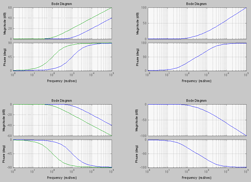
The figure below shows the plots of two first order systems corner frequencies
 and
and
 , together with the plots of their product, a
second order system.

- Second-order factor
 |
(514) |
The denominator is a 2nd order polynomial for variable  . Consider the
following two cases:
First, if
 i.e., if
 , the denominator has two real and negative roots:
 |
(515) |
and
 can be written as a product of two first order FRFs:
 |
(516) |
where
 and
and
 are the two time constant of the two
first order systems. Now the second order factor is the product of two first order
factors and
 |
(517) |
with corner frequencies at
 and
and
 .
.
Second, if  , i.e., the two roots are complex. We consider the numerator
and the denominator separately. The numerator is just a constant with zero phase and
log-magnitude of
 . Next consider the
rest of the function:
![$\displaystyle \vert H(j\omega)\vert=[(1-(\frac{\omega}{\omega_n})^2)^2+(2\zeta\frac{\omega}{\omega_n})^2]^{-1/2
}$](img1421.svg) |
(518) |
We have
| |
|
![$\displaystyle Lm\;H(j\omega)=20\log_{10} \vert H(j\omega)\vert
=-10\;\log_{10}[\; (1-(\frac{\omega}{\omega_n})^2)^2+(2\zeta\frac{\omega}{\omega_n})^2\;]$](img1422.svg) |
(519) |
 |
(520) |
Consider three cases:
-
 :
Now
:
Now
 and
and
 |
(521) |
-
 , i.e.,
 :
:
 |
(522) |
-
 , i.e.,
 :
:
![$\displaystyle Lm\;H(j\omega)\approx-10\;\log_{10}[\; (\frac{\omega}{\omega_n})^4 ]
=-40 \;\log_{10} \frac{\omega}{\omega_n}$](img1431.svg) |
(523) |
This is a straight line with slop of -40 dB per decade.
 |
(524) |


 :
:

 ,
,

 becomes ten times higher, then

 is a straight line with a slop of 20 dB/dec that goes
through a zero-crossing at
  .
.


 . For example, when
  , we have:


 :
:

 is a straight line with a slop of -20 dB/dec that goes
through a zero-crossing at
  .
.


 , i.e.,
 is the corner frequency, we have

 (e.g.,
 ):
):

 (e.g.,
 ):
):

 has zero slope when
 but a slope 20 dB/dec when
 . The straight-line asymptote of
 is zero when
 ,
,  when
when
 ,
but with a slope
 in between.


 is simply the negative
version of
 .
.


 . Consider the
following two cases:


 can be written as a product of two first order FRFs:

 and
and
 are the two time constant of the two
first order systems. Now the second order factor is the product of two first order
factors and

 and
and
 .
.


![$\displaystyle \vert H(j\omega)\vert=[(1-(\frac{\omega}{\omega_n})^2)^2+(2\zeta\frac{\omega}{\omega_n})^2]^{-1/2
}$](img1421.svg)
![$\displaystyle Lm\;H(j\omega)=20\log_{10} \vert H(j\omega)\vert
=-10\;\log_{10}[\; (1-(\frac{\omega}{\omega_n})^2)^2+(2\zeta\frac{\omega}{\omega_n})^2\;]$](img1422.svg)

 :
Now
:
Now
 and
and

 , i.e.,
 :
:

 , i.e.,
 :
:
![$\displaystyle Lm\;H(j\omega)\approx-10\;\log_{10}[\; (\frac{\omega}{\omega_n})^4 ]
=-40 \;\log_{10} \frac{\omega}{\omega_n}$](img1431.svg)


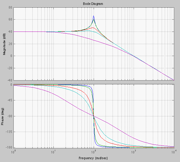
 . When
  i.e.,
i.e.,
 , we have

 is not at
  , but at the resonant frequency
 , which can be found by taking derivative of the magnitude of the denominator
with respect to
  and setting it to zero:
![$\displaystyle \frac{d}{du}[u^2+(4\zeta^2-2)u+1]=2u+4\zeta^2-2=0$](img1438.svg)
 i.e.,
i.e.,
 , the peak is:

 , i.e.,
 , the result is complex indicating there
is no peak.