Second-order system as a filter

Consider a second order circuit of the series combination of R, C, and L, connected to an input voltage source $v_0(t)$. We can treat any of the voltages $v_R(t)$, $v_C(t)$, and $v_L(t)$, across R, C, and L, respectively as the output. The second order system can be used as a band-pass (BP), high-pass (HP), or low-pass (LP) filter, if the voltage across R, L, or C is treated as the output. In general, the resonant frequency $\omega_r$ of a system is the frequency at which the magnitude of its frequency response function is maximized. In the following, we specifically consider the magnitude of the frequency response function (FRF) of these filters. In particular, we will consider $\vert H(\omega)\vert$ when $\omega=0$, $\omega=\omega_r$, $\omega=\omega_n$, and $\omega=\infty$.

• 2nd-order Band-pas Filter:

  If the voltage across $R$ is treated as the output, we have

  $$\dot{V}_R=\dot{V}_0\;\frac{Z_R}{Z_R+Z_C+Z_L} =\dot{V}_0\;\frac{R}{R+1/j\omega C+j\omega L} =\dot{V}_0\;\frac{R}{R+j(\omega L-1/\omega C)}$$ (320)

  The FRF of the system is
  

  $$H_R(\omega) = \frac{R}{R+j\omega L+1/j\omega C} =\frac{R \;j\omega/L}{(R+j\omega L+1/j\omega C)\;j\omega/L}$$

  $$= \frac{j\omega R/L}{j\omega R/L+(j\omega)^2+1/LC} =\frac{j\omega 2\zeta \omega_n}{(j\omega)^2 +j\omega 2\zeta \omega_n+\omega_n^2}$$ (321)

  
  

  At the natural frequency $\omega=\omega_n=1/\sqrt{LC}$, the imaginary part of the denominator $\omega_n L-1/\omega_n C=0$ is zero and $H_R(\omega_n)=1$ is the maximum, i.e., the resonant frequency is the same as the natural frequency $\omega_r=\omega_n=1/\sqrt{LC}$. When $\omega\ne \omega_n$, we have $\vert H_R(\omega)\vert<\vert H_R(\omega_n)\vert$. In particular:

  • $\vert H_R(0)\vert=0$
  • $\vert H_R(\omega_n)\vert=\vert H_R(\omega_r)\vert=1$
  • $\vert H_R(\infty)\vert=0$

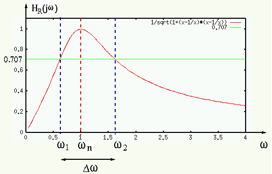
  This is a band-pass filter with the bandwidth defined as:

  $$\triangle \omega=\omega_2-\omega_1$$ (322)

  where $\omega_1<\omega_r$ and $\omega_2>\omega_r$ are the two cut-off frequencies at which

  $$\vert H(\omega_1)\vert=\vert H(\omega_2)\vert=\frac{1}{\sqrt{2}}=0.707,\;\;\;\;\; \;\;\;\;\;\;\vert H(\omega_1)\vert^2=\vert H(\omega_2)\vert^2=\frac{1}{2}$$ (323)

  In other words, the power of the output is halved when compared to that of the input. The cut-off frequency is therefore also called the half-power frequency. To find the bandwidth of this 2nd order system, we rewrite the FRF as:

  $$H_R(\omega)=\frac{R}{R+j\omega L+1/j\omega C} =\frac{1}{1+j(\omega L/R-1/\omega RC)}$$ (324)

  Note that $\vert H_R(\omega)\vert=1/\sqrt{2}$ when the imaginary part of the denominator is:

  $$\frac{\omega L}{R}-\frac{1}{\omega CR}=\pm 1$$ (325)

  To solve this equation for the cut-off frequency, we multiply both sides by $\omega R/L$, and get two quadratic equations:

  $$\omega^2\pm \frac{R}{L}\omega-\frac{1}{LC}=\omega^2\pm 2\zeta\omega_n\omega-\omega_n^2=0$$ (326)

  with four roots:

  $$\omega=\frac{1}{2}\left(\mp 2\zeta\omega_n\pm\sqrt{4\zeta^2\omega_n^2+4\omega_n^2}\right) =\left(\mp\zeta\pm\sqrt{\zeta^2+1}\right)\omega_n$$ (327)

  Ignoring the negative roots (with no physical meaning) we get the two cut-off frequencies $\omega_1$ and $\omega_2$:

  $$\omega_{1,2}=\left(\sqrt{1+\zeta^2}\mp \zeta\right) \omega_n$$ (328)

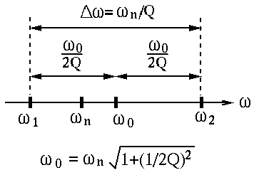
  and the bandwidth is

  $$\triangle \omega=\omega_2-\omega_1=2\zeta \omega_n=\frac{\omega_n}{Q} =\frac{R}{L}$$ (329)

  This happens to be the coefficient of the first order term in the canonical form of the second order system, which can now be written as:

  $$y''(t)+2\zeta\omega_n\,y'(t)+\omega_n^2\, y(t) =y''(t)+\triangle\omega\,y'(t)+\omega_n^2\, y(t)= x(t)$$ (330)

  The equation $\triangle\omega=\omega_n/Q$ is of great importance as it directly relates the bandwidth $\Delta\omega$ and the natural frequency $\omega_n$.

  The middle point between the two cut-off frequencies $\omega_1$ and $\omega_2$ is

  $$\omega_0=\frac{\omega_1+\omega_2}{2} =\omega_n \sqrt{1+\zeta^2}\;>\;\omega_n$$ (331)

  which is greater than the resonant frequency $\omega_r=\omega_n$, and we have $\omega_2-\omega_n>\omega_n-\omega_1$.

  

  

  If $Q=1/2\zeta \gg 1$ (typically $Q>10$, i.e., $\zeta<0.05$), we have $\sqrt{1+\zeta^2} =\sqrt{1+(1/2Q)^2} \approx 1$, $\omega_0\approx\omega_n$, and

  $$\omega_{1,2}\approx \omega_n\mp \frac{\triangle\omega}{2} =\omega_n\mp\frac{2\zeta\omega_n}{2}=\omega_n(1\mp\zeta)$$ (332)

  $$H_{bp}(\omega)=\frac{j\omega 2\zeta \omega_n}{(j\omega)^2 +j\omeg... ...=\frac{j\omega \triangle \omega} {\triangle \omega j\omega+\omega_n^2-\omega^2}$$ (333)

• 2nd-order High-pass Filter:

  If the voltage across $L$ is treated as the output, we have
  

  $$H_L(\omega) = H_{hp}(\omega)=\frac{j\omega L}{R+j\omega L+1/j\omega C} =\frac{j\omega L\;j\omega/L}{(R+j\omega L+1/j\omega C)\;j\omega/L}$$

  $$= \frac{(j\omega)^2}{(j\omega)^2+j\omega 2\zeta \omega_n+\omega_n^2... ...n^2-\omega^2} %\;\;\;\;\;\;H(s)=\frac{s^2}{s^2+\triangle\omega s +\omega_n^2}$$ (334)

  
  This is a high-pass filter as
  • $\vert H(0)\vert=0$
  • $\vert H(\omega_n)\vert=1/2\zeta=Q$
  • $\vert H(\infty)\vert=1$
  To decide whether $H_L(\omega)$ peaks and, if so, to find the resonant frequency, we consider
  

  $$\vert H_{lp}(\omega)\vert^2 = \frac{\omega^4}{(2\zeta\omega_n\omega)^2+(\omega_n^2-\omega^2)^2} =\frac{\omega^4}{\omega^4-(1-2\zeta^2)2\omega_n^2\omega^2+\omega_n^4}$$ (335)

  
  and set its derivative with respect to $\omega$ to zero:
  

  $$\frac{d}{d\omega}\vert H_{hp}(\omega)\vert^2 = \frac{d}{d\omega}\left[\frac{\omega^4}{(\omega_n^2-\omega^2)^2 +(2\zeta\omega\omega_n)^2}\right]$$

  $$= \frac{4\omega^3[(\omega_n^2-\omega^2)^2+4\zeta^2\omega^2\omega_n^... ...^2\omega\omega_n^2]}{[(\omega_n^2-\omega^2)^2+4\zeta^2\omega^2\omega_n^2]^2} =0$$ (336)

  
  For this equation to hold, the numerator needs to be zero:

  $$4\omega^3[(\omega_n^2-\omega^2)^2+4\zeta^2\omega^2\omega_n^2] =4\omega^5[\omega^2-\omega^2_n+2\zeta^2\omega_n^2]$$ (337)

  Solving this for $\omega$, we get the resonant frequency:

  $$\omega_r=\frac{\omega_n}{\sqrt{1-2\zeta^2}}$$ (338)

  Now consider the following three cases:
  • If $\zeta<1/\sqrt{2}$, i.e., $Q>1/\sqrt{2}$, then $\omega_r>\omega_n$ is real and $\vert H_L(\omega)\vert$ peaks at $\omega_r$:

    $$\vert H_{hp}(\omega_r)\vert=\frac{1}{2\zeta\sqrt{1-\zeta^2}} =\frac{2Q^}{\sqrt{4Q^2-1}} >\vert H_{hp}(\omega_n)\vert=\frac{1}{2\zeta}=Q$$ (339)

    If $\zeta$ is small, $\omega_r\approx\omega_n$. For example, $\zeta=0.05$, $\omega_r=1.0025\,\omega_n$.

  • If $\zeta=Q=1/\sqrt{2}$, then $\omega_r=\infty$, and

    $$\vert H_{hp}(\omega_n)\vert=\frac{1}{\sqrt{2}}\;<\; \vert H_{hp}(\omega_r)\vert\; =\;\vert H_{lp}(\infty)\vert=\;1$$ (340)

    or $20\log \vert H_{hp}(\omega_n)\vert=-3\,dB$, i.e., $\omega_n$ is the cut-off frequency of the HP filter.
  • If $\zeta>1/\sqrt{2}$, $\omega_r$ is imaginary, indicating there does not exist a frequency at which $H_L(\omega)$ peaks.

• 2nd-order Low-pass Filter:

  If the voltage across $C$ is treated as the output, we have
  

  $$H_C(\omega) = H_{lp}(\omega)=\frac{1/j\omega C}{R+j\omega L+1/j\omega C} =\frac{1/j\omega C\;j\omega/L}{(R+j\omega L+1/j\omega C)\;j\omega/L}$$

  $$= \frac{\omega_n^2}{(j\omega)^2+j\omega 2\zeta \omega_n+\omega_n^2}... ...ega^2} %\;\;\;\;\;\;H(s)=\frac{\omega_n^2}{s^2+\triangle\omega s +\omega_n^2}$$ (341)

  
  This is a low-pass filter as
  • $\vert H(0)\vert=1$
  • $\vert H(\omega_n)\vert=1/2\zeta=Q$
  • $\vert H(\infty)\vert=0$
  To decide whether $H_L(\omega)$ peaks and, if so, to find the resonant frequency, we consider

  $$\vert H_{lp}(\omega)\vert^2 =\frac{\omega_n^4}{(2\zeta\omega_n\om... ...a^2)^2} =\frac{\omega_n^4}{\omega^4-(1-2\zeta^2)2\omega_n^2\omega^2+\omega_n^4}$$ (342)

  To find $\omega_r$ that maximizes $\vert H_C(\omega)\vert^2$ or equivalently minimizes its denominator (with constant numerator), we set the derivative of the denominator with respect to $\omega$ to zero:
  

  $$\frac{d}{d\omega}\bigg\vert(j\omega)^2+j\omega 2\zeta\omega_n+\omega^2\bigg\vert^2 = \frac{d}{d\omega} [(\omega_n^2-\omega^2)^2+4\zeta^2\omega_n^2\omega^2]$$

  $$= -4\omega(\omega_n^2-\omega^2)+8\zeta^2\omega_n^2\omega=0$$ (343)

  
  Solving for $\omega$ we get the resonant frequency:

  $$\omega_r=\omega_n\sqrt{1-2\zeta^2}<\omega_n$$ (344)

  Now consider the following three cases:
  • If $\zeta<1/\sqrt{2}$, i.e., $Q<1/\sqrt{2}$, then $\omega_r<\omega_n$ is real and $\vert H_C(\omega)\vert$ peaks at $\omega_r$:

    $$\vert H_{lp}(\omega_r)\vert=\frac{1}{2\zeta\sqrt{1-\zeta^2}} =\frac{2Q^2}{\sqrt{4Q^2-1}} \;>\; \vert H_{lp}(\omega_n)\vert=\frac{1}{2\zeta}=Q$$ (345)

    If $\zeta$ is small, $\omega_r\approx\omega_n$. For example, $\zeta=0.05$, $\omega_r=0.9975\,\omega_n$.

  • If $\zeta=Q=1/\sqrt{2}$, we have $\omega_r=0$, and

    $$\vert H_{lp}(0)\vert\;=\;\vert H_{lp}(\omega_r)\vert=1>\vert H_{lp}(\omega_n)\vert =\frac{1}{\sqrt{2}}$$ (346)

    or $20\log \vert H_{lp}(\omega_n)\vert=-3\,dB$, i.e., $\omega_n$ is the cut-off frequency of the LP filter.
  • If $\zeta>1/\sqrt{2}$, $\omega_r$ is imaginary, indicating there does not exist a frequency at which $H_C(\omega)$ peaks.

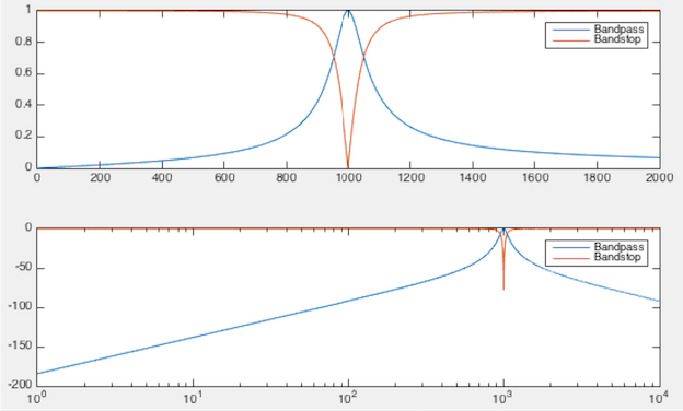
At the natural frequency, the impedance of a series RCL circuit reaches minimum, consequently the current reaches maximum and so does the voltage across the resistor. However, the voltage across the inductor reaches maximum at a frequency slightly higher than the natural frequency, and the voltage across the capacitor reaches maximum at a frequency slightly lower than the resonant frequency, as shown in the linear and log-scale plots below. (For Bode plots, see here.)

In summary,

• Low-pass filter:

  $$H_{lp}=\frac{Z_C}{Z_C+Z_R+Z_L} =\frac{\omega_n^2}{(j\omega)^2+\triangle \omega j\omega+\omega_n^2}$$ (347)

• High-pass filter:

  $$H_{hp}=\frac{Z_L}{Z_C+Z_R+Z_L} =\frac{(j\omega)^2}{(j\omega)^2+\triangle \omega j\omega+\omega_n^2}$$ (348)

• Band-pass filter:

  $$H_{bp}=\frac{Z_R}{Z_C+Z_R+Z_L} =\frac{\triangle\omega j\omega}{(j\omega)^2+\triangle \omega j\omega+\omega_n^2}$$ (349)

• Band-stop filter:

  $$H_{bs}=\frac{Z_C+Z_L}{Z_C+Z_R+Z_L} =\frac{\omega_n^2+(j\omega)^2}{(j\omega)^2+\triangle \omega j\omega+\omega_n^2}$$ (350)

• All-pass filter:

  $$H_{ap}=\frac{Z_C+Z_R+Z_L}{Z_C+Z_R+Z_L} =\frac{(j\omega)^2+\triangle \omega j\omega+\omega_n^2}{(j\omega)^2+\triangle \omega j\omega+\omega_n^2}$$ (351)

For a parallel RCL circuit with current input, due to the duality between current and voltage, parallel and series configuration, the same derivation of bandwidth can be carried out to obtain the same conclusions.

While the phenomenon of resonance can be destructive in mechanical systems (for example, the famous story of the Angers bridge), and it therefore needs to be avoided, it can also be very useful in electrical system such as in the tuning circuit in radio or TV broadcasting.

Example: Given the RLC circuits below, find what kind of filters they are (HP, LP, BP, or BS).

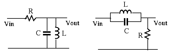
The impedance of the parallel combination of $L$ and $C$ is:

$$Z_{LC}=Z_C\vert\vert Z_L=\frac{Z_LZ_C}{Z_L+Z_C} =\frac{j\omega L/... ...a C} =\frac{j\omega L}{1-\omega^2 LC} =\frac{j\omega L}{1-(\omega/\omega_n)^2 }$$ (352)

At the resonant frequency $\omega=\omega_n=1/\sqrt{LC}$, $Z_{LC}=\infty$ (open-circuit):

$$\vert Z_{LC}\vert=\left\{\begin{array}{cc}0 & \omega=0\\ \infty & \omega=\omega_n\\ 0 & \omega=\infty\end{array}\right.$$ (353)

• The FRF of the first circuit is

  $$H_{LC}=\frac{Z_{LC}}{Z_{LC}+R}=\frac{\frac{j\omega L}{1-(\omega/\... ...-(\omega/\omega_n)^2)} =\frac{1}{1-j\frac{(1-(\omega/\omega_n)^2)}{\omega L/R}}$$ (354)

  When $\omega=\omega_n$, $Z_{LC}=\infty$, $H_{LC}=1$. In this case no current goes through $R$ and the voltage drop across it is zero, then the output voltage is the same as the input voltage. Otherwise either $\omega>\omega_n$ or $\omega<\omega_n$, $Z_{LC}$ is finite, the voltage across $R$ is non-zero, the output voltage is reduced. This is a band-pass filter:

  $$\vert H_{BP}\vert=\bigg\vert\frac{Z_C\vert\vert Z_L}{R+Z_C\vert\v... ...rightarrow 0\\ 1&\omega=\omega_n\\ 0&\omega\rightarrow\infty\end{array}\right.$$ (355)

• The FRF of the second circuit is

  $$H_R=\frac{R}{Z_{LC}+R}=\frac{R}{\frac{j\omega L}{1-(\omega/\omega_n)^2}+R} =\frac{1}{j\,\frac{\omega L/R}{1-(\omega/\omega_n)^2 }+1}$$ (356)

  when $\omega=\omega_n$, $Z_{LC}=\infty$, $H_R=0$. In this case, the LC parallel branch is an open-circuit, the output voltage is zero. Otherwise either $\omega>\omega_n$ or $\omega<\omega_n$, $Z_{LC}$ is finite, the voltage is non-zero. The circuit is a band-stop or band-block filter:

  $$\vert H_{BS}\vert=\bigg\vert\frac{R}{R+Z_C\vert\vert Z_L}\bigg\ve... ...rightarrow 0\\ 0&\omega=\omega_n\\ 1&\omega\rightarrow\infty\end{array}\right.$$ (357)

Example: Find the bandwidth of each of the two filters above as a function of $R$, $C$ and $L$. Determine whether the peak frequency $\omega_n$ is lower or higher than the center of the passing/stop band. Design a band-pass and a band-stop filter so that the peak frequency is $\omega_n=1000$ and the bandwidth is $\Delta\omega=100$.

The bandwidth is defined as $\Delta\omega=\omega_2-\omega_1$, the difference between the two cut-off frequencies $\omega_1<\omega_n$ and $\omega_2>\omega_n$ at which $\vert H\vert=1/\sqrt{2}$. For both filters, the cut-off frequencies can be found by solving

$$1-\left(\frac{\omega}{\omega_n}\right)^2 =\pm \frac{\omega L}{R}$$ (358)

i.e., the two filters always have the same bandwidth.

$$1-\omega^2LC=\pm \omega L/R,\;\;\;\;\; \omega^2\pm\frac{1}{RC}\omega-\frac{1}{LC}=0$$ (359)

Solving these two quadratic equations and take the positive roots of each, we get

$$\omega_{1,2}=\frac{1}{2}\left(\sqrt{\frac{1}{R^2C^2}+\frac{4}{LC}}\pm \frac{1}{RC}\right)$$ (360)

The bandwidth is

$$\Delta\omega=\omega_2-\omega_1=\frac{1}{RC}$$ (361)

The center of the bandwidth is greater than peak frequency:

$$\frac{\omega_1+\omega_2}{2}=\frac{1}{2}\sqrt{\frac{1}{R^2C^2}+\frac{4}{LC}} >\frac{1}{\sqrt{LC}}=\omega_n$$ (362)

Given the desired properties:

$$\omega_n=\frac{1}{\sqrt{LC}}=10^3,\;\;\;\;\;\;\;\Delta\omega=\frac{1}{RC}=10^2$$ (363)

we further get

$$LC=10^{-6},\;\;\;\;\;\;\;\;\;\;\;\;\;\;RC=10^{-2}$$ (364)

If we let $R=100$, then we get $C=10^{-4}\;F$, $L=10^{-2}\;H$, and

$$\omega_n=\frac{1}{\sqrt{LC}}=\frac{1}{\sqrt{10^{-6}}}=10^3, \;\;\;\;\; \Delta\omega=\frac{1}{RC}=\frac{1}{10^{-2}}=100$$ (365)