First-order system as a filter

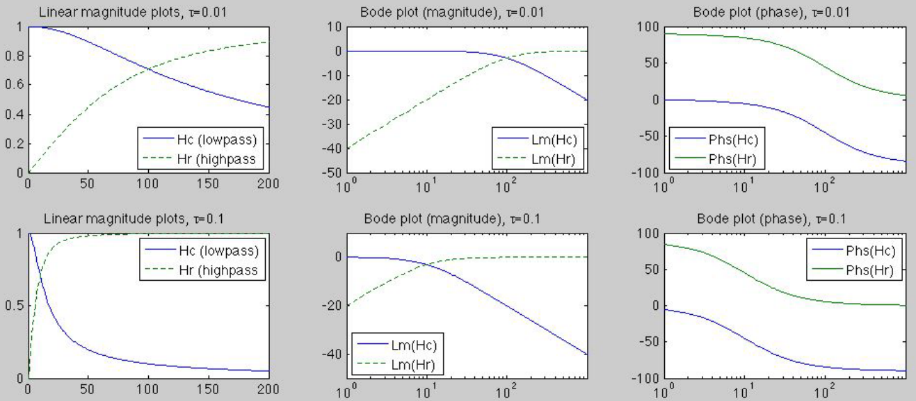
The first order RC and RL systems can be used as either a high-pass or low-pass filter, depending on voltage across which component is treated as the output, while the input voltage $v_0(t)$ is applied across both components connected in series. For example, if the voltage $v_R(t)$ across $R$ is treated as the output, the RC circuit is a high-pass filter and the RL circuit is a low-pass filter. The cut-off or corner frequency of such filters is $\omega_c=1/\tau$.

• RC circuit

  Treating the RC circuit as a voltage divider, the phasor representations of the voltage across $R$ and $C$ are

  $$\dot{V}_R=\dot{V}_0\frac{R}{R+1/j\omega C}=\dot{V}_0\frac{j\omega RC}{j\omega RC+1} =\dot{V}_0\frac{j\omega\tau}{j\omega\tau+1}$$ (309)

  and

  $$\dot{V}_C=\dot{V}_0\frac{1/j\omega_c}{R+1/j\omega C} =\dot{V}_0\frac{1}{1+j\omega RC}=\dot{V}_0\frac{1}{1+j\omega\tau}$$ (310)

  where $\tau=RC$ is the time constant of this RC first order system. The FRFs and transfer functions of the systems are

  $$H_R(\omega)=\frac{\dot{V}_R}{\dot{V}_0}=\frac{j\omega\tau}{j\omega\tau+1}$$ (311)

  $$H_C(\omega)=\frac{\dot{V}_C}{\dot{V}_0}=\frac{1}{1+j\omega\tau}$$ (312)

  $H_R$ and $H_C$ are high-pass and low-pass filters, respectively. At the cut-off frequency defined as $\omega_c=1/\tau=1/RC$, the magnitude of the output attenuates to $1/\sqrt{2}$ of the peak magnitude, the output power is half of the input power:

  $$\vert H_R(\omega)\vert=\left\{\begin{array}{cl}0&\omega=0\\ 1/\s... ...mega=0\\ 1/\sqrt{2}&\omega=\omega_c=1/\tau\\ 0&\omega=\infty\end{array}\right.$$ (313)

• RL circuit

  Treating the RL circuit as a voltage divider, the phasor representation of the voltage across $R$ can be found to be

  $$\dot{V}_R=\dot{V}_0\frac{R}{R+j\omega L} =\dot{V}_0\frac{1}{1+j\omega L/R}=\dot{V}_0\frac{1}{1+j\omega\tau}$$ (314)

  $$\dot{V}_L=\dot{V}_0\frac{j\omega L}{R+j\omega L} =\dot{V}_0\frac{... ...{V}_0\frac{j\omega}{j\omega+1/\tau} =\dot{V}_0\frac{j\omega\tau}{j\omega\tau+1}$$ (315)

  where $\tau=L/R$ is the time constant of this RL first order system. The FRFs and transfer functions of the system are

  $$H_R(\omega)=\frac{\dot{V}_R}{\dot{V}_0}=\frac{1}{j\omega\tau+1}$$ (316)

  $$H_L(\omega)=\frac{\dot{V}_L}{\dot{V}_0}=\frac{j\omega\tau}{j\omega\tau+1}$$ (317)

  and

  $$\vert H_R(\omega)\vert=\left\{\begin{array}{cl}0&\omega=\infty\\ 1/\sqrt{2}&\omega=\omega_c=1/\tau\\ 1&\omega=0\end{array}\right.$$ (318)

  This system is a low-pass filter as it passes low frequencies but attenuates high frequencies.

The cut-off or corner frequency $\omega_c=1/\tau=L/R$ is defined as the frequency at which the magnitude of the output attenuates to $\vert H(\omega_c)\vert=1/\sqrt{2}$ of the peak magnitude, unity in first order systems, and the output power is half of the peak power, the input power for first order systems. The gain of a system is typically measured in decibel (dB) and plotted in Bode plots in terms of the log-magnitude of the FRF defined as $20 \log_{10}\vert H(\omega)\vert$. At the cut-off frequency, we have

$$20 \log_{10}(1/\sqrt{2})=-20\log_{10}\sqrt{2}=-10\log_{10}2=-3$$ (319)

(For more discussion of the Bode plots, see here.)