Next: Stability Analysis of Nonlinear
Up: DEsystem
Previous: Matrix Exponential Function
Now we consider the general solution of a nonhomogeneous ODE system
with non-zero input  on the right-hand side:
Multiply both sides by  :
:
Integrate both sides
Multiply  on both side:
where the first term
 is the
homogeneous solution of the ODE system
is the
homogeneous solution of the ODE system
 , and
the second term is the particular solution.
, and
the second term is the particular solution.
Example 1:
Define  ,
,
or in matrix form:
Given  and
and  , we have
with eigenvalue and eigenvector matrices:
Given  and
and  , we get
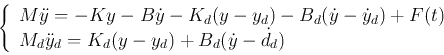
Example 2:
The motion of a tuned mass damper system
shown below:
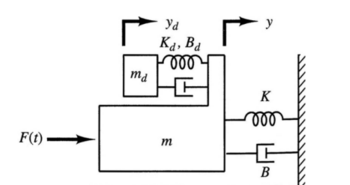
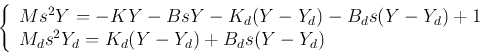
can be described by the following two ODEs:
If we define and  , then we get
and we have
which can be written in matrix form as
where
![${\bf x}=[0,\;\delta(t)/M,\;0,\;0]^T$](img129.png) .
.
We assume zero initial condition
 and
and
 , and
, and
 , then
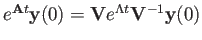
we get the solution
, then
we get the solution
The first component of  is:
is:
which is the 1st row and 2nd column of
 ;
and the third component of is:
;
and the third component of is:
which is the 3rd row and 2nd column of
;
The problem can also be solved using the Laplace transform method.
Let
![$Y(s)={\cal L}[\;y(t)\;]$](img137.png) and
and
![$Y_d(s)={\cal L}[\;y_d(t)\;]$](img138.png) , then
, then
![${\cal L}[\;\dot{y}(t)\;]=s Y(s)-y(0)=s Y(s)$](img139.png) and
and
![${\cal L}[\;\ddot{y}(t)\;]=s^2 Y(s)$](img140.png)
![${\cal L}[\;\dot{y}_d(t)\;]=s Y_d(s)$](img141.png)
![${\cal L}[\;\ddot{y}_d(t)\;]=s^2 Y_d(s)$](img142.png) .
.
Now the two DEs can be expressed in s-domain as:
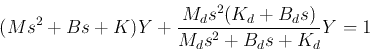
Find the sum of the two equations:
and rewrite the second equation as:
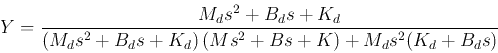
Substituting into the other equation we get
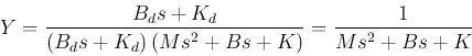
Solving for  we get
Note that when  , the system becomes a regular damped harmonic
oscillator:
, the system becomes a regular damped harmonic
oscillator:
The motion of mass  is:
is:
Next: Stability Analysis of Nonlinear
Up: DEsystem
Previous: Matrix Exponential Function
Ruye Wang
2019-02-21
![\begin{displaymath}
\frac{d}{dt}\left[\begin{array}{c}y v\end{array}\right]
\l...
...rray}\right]+
\left[\begin{array}{c}0 x(t)\end{array}\right]
\end{displaymath}](img115.png)
![\begin{displaymath}
{\bf A}=\left[\begin{array}{cc}0 & 1 100 & 0\end{array}\right]
\end{displaymath}](img119.png)
![\begin{displaymath}
{\bf D}=\left[\begin{array}{cc}10 j & 0 0 & -10\;j\end{ar...
...left[\begin{array}{cc}1 & 1 10 j & -10\;j\end{array}\right]
\end{displaymath}](img120.png)
![\begin{displaymath}
e^{{\bf A}t}={\bf V}e^{{\bf D}t}{\bf V}^{-1}
=\left[\begin{a...
...10 t)/10\\
-10 \sin(10 t) & \cos(10 t) \end{array}\right]
\end{displaymath}](img121.png)
![\begin{displaymath}
y(t)=[1\;0]e^{{\bf A}t}\left[\begin{array}{c}0\ 1\end{array...
...f A}t}
\left[\begin{array}{c}0\ x(t)\end{array}\right]\;d\tau
\end{displaymath}](img124.png)
![\begin{displaymath}
\left\{
\begin{array}{l}
\dot{v}=\ddot{y}=[-Ky-B\dot{y}-K_d(...
...}_d=[K_d(y-y_d)+B_d(\dot{y}-\dot{d}_d)]/M_d
\end{array}\right.
\end{displaymath}](img127.png)
![\begin{displaymath}
\frac{d}{dt}\left[\begin{array}{d}y v y_d v_d\end{arra...
...t[\begin{array}{d}0 \frac{F(t)}{M} 0 0\end{array}\right]
\end{displaymath}](img128.png)
![\begin{displaymath}
{\bf y}={e^{\bf A}t}{\bf y}(0) {\bf Ay}+\int_0^te^{{\bf A}\t...
...A}t}\left[\begin{array}{c} 0 1/M 0 0 \end{array} \right]
\end{displaymath}](img133.png)
![\begin{displaymath}
y(t)=[1\;0\;0\;0]\;{\bf y}(t)=[1\;0\;0\;0]
e^{{\bf A}t}\left[\begin{array}{c} 0 1/M 0 0 \end{array} \right]
\end{displaymath}](img134.png)
![\begin{displaymath}
y_d(t)=[0\;0\;1\;0]\;{\bf y}(t)=[0\;0\;1\;0]
e^{{\bf A}t}\left[\begin{array}{c} 0 1/M 0 0 \end{array} \right]
\end{displaymath}](img136.png)