Matrix Exponential Function

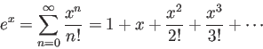
Based on the Taylor expansion of the exponential function of a scalor variable:

$$e^x=\sum_{n=0}^\infty \frac{x^n}{n!}=1+x+\frac{x^2}{2!}+\frac{x^3}{3!}+\cdots$$

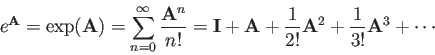
we can also define the exponential function of a matrix ${\bf A}$ as

$$e^{\bf A}=\exp({\bf A})=\sum_{n=0}^\infty \frac{{\bf A}^n}{n... ... I}+{\bf A}+\frac{1}{2!}{\bf A}^2+\frac{1}{3!}{\bf A}^3+\cdots$$

In particular, when ${\bf A}={\bf0}$, we get $\exp({\bf0})={\bf I}$.

Consider the eigenequation of ${\bf A}$:

$${\bf Av}_i=\lambda_i{\bf v}_i,\;\;\;\;\;\;\;(i=1,\cdots,n)$$

These $n$ equations can be combined to become

$${\bf AV}={\bf A}[{\bf v}_1,\cdots,{\bf v}_n]=[{\bf v}_1,\cdo... ...s&\vdots 0&\cdots&\lambda_n\end{array}\right]={\bf V\Lambda}$$

we therefore also have

$${\bf A}={\bf V\Lambda V}^{-1},\;\;\; {\bf A}^2=({\bf V\Lambd... ...{-1},\;\;\; {\bf A}^3={\bf V\Lambda}^3{\bf V}^{-1}\cdots\cdots$$

i.e., in general,

$${\bf A}^n={\bf V\Lambda}^n{\bf V}^{-1}$$

Now r$\exp({\bf A})$ can be written as:

$$\exp({\bf A}) = \exp({\bf V\Lambda V}^{-1})={\bf I}+{\bf V\Lambda V}^{-1} +\frac... ...2!}{\bf V\Lambda}^2{\bf V}^{-1}+\frac{1}{3!}{\bf V\Lambda}^3{\bf V}^{-1}+\cdots$$

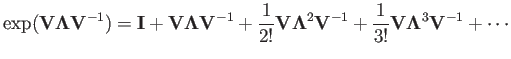
$$= {\bf V}\left[{\bf I}+{\bf\Lambda}+\frac{1}{2!}{\bf\Lambda}^2+\fra... ...}{\bf\Lambda}^3 +\cdots\right]{\bf V}^{-1} ={\bf V}e^{\bf\Lambda}{\bf V}^{-1}$$

$$= {\bf V}\left[\begin{array}{ccc}e^{\lambda_1}&\cdots&0 \vdots&\ddots&\vdots 0&\cdots&e^{\lambda_n}\end{array}\right]{\bf V}^{-1}$$