Next: Matrix Exponential Function
Up: DEsystem
Previous: Differential Equation System
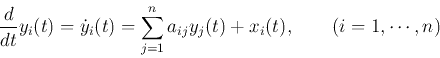
Consider solving a set of  first order constant coefficient ordinary
differential equations (ODE):
first order constant coefficient ordinary
differential equations (ODE):
which can be written in matrix form:
where
In particular, if
 , we get a homogeneous ODE system:
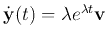
We let the solution take the form of
 ,
where scalor
,
where scalor  and vector
  are to be determined. We
then have e
are to be determined. We
then have e
 . Substituting
these into the DE system we get
. Substituting
these into the DE system we get
Dividing both sides by
 , we get:
This happens to be the eigenequation of  , and
and can be found as the eigenvalue and the corresponding
eigenvector of . In general, solving this equation we get
eigenvalues
, and
and can be found as the eigenvalue and the corresponding
eigenvector of . In general, solving this equation we get
eigenvalues
 and their corresponding
eigenvectors
and their corresponding
eigenvectors
 . We therefore get a set of
fundamental solutions
. We therefore get a set of
fundamental solutions
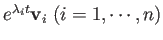 of
the ODE system, all satisfying
of
the ODE system, all satisfying
These equations can be combined to become
where
are the eigenvalue and eigenvector matrices of .
The fundamental matrix of the ODE system
 is a matrix of which each column is a solution:
The general solution of the ODE system is a linear combination of
the fundamental solutions
where
![${\bf c}=[c_1,\cdots,c_n]^T$](img73.png) is a vector containing
coefficients, which can be found based on the given initial
conditions
is a vector containing
coefficients, which can be found based on the given initial
conditions
![${\bf y}(0)=[y_1(0),\cdots,y_n(0)]^T$](img74.png) . Specifically,
evaluating the solution
. Specifically,
evaluating the solution  at
at  , we get
Solving the equation
 we get the coefficients:
Substituting this  back into the general solution above,
we finally get the homogeneous solution of the ODE system:
back into the general solution above,
we finally get the homogeneous solution of the ODE system:
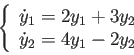
Example
Solve the following DE
with initial conditions  and
and  . The coefficient
matrix is
. The coefficient
matrix is
and its eigenvalues are  and
and  and their
corresponding eigenvectors are
and their
corresponding eigenvectors are
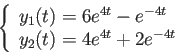
The solution is
The coefficients can be found by
The solution is
i.e.,
Next: Matrix Exponential Function
Up: DEsystem
Previous: Differential Equation System
Ruye Wang
2019-02-21
![\begin{displaymath}
{\bf x}=\left[\begin{array}{c}x_1 \vdots x_n\end{array}\...
...& \ddots & \vdots a_{n1} & \cdots &a_{nn}\end{array}\right]
\end{displaymath}](img53.png)
![\begin{displaymath}
{\bf A}[{\bf v}_1,\cdots,{\bf v}_n]=[{\bf v}_1,\cdots,{\bf v...
...ight]
\;\;\;\;\;\;\mbox{or}\;\;\;\;\;\;{\bf AV}={\bf V\Lambda}
\end{displaymath}](img68.png)
![\begin{displaymath}
{\bf\Lambda}=\left[\begin{array}{ccc}\lambda_1&\cdots&0 \...
...ray}\right],\;\;\;\;\;\;
{\bf V}=[{\bf v}_1,\cdots,{\bf v}_n]
\end{displaymath}](img69.png)
![\begin{displaymath}[e^{\lambda_1t}{\bf v}_1,\cdots,e^{\lambda_nt}{\bf v}_n]
=[{\...
...\cdots&e^{\lambda_nt}\end{array}\right]
={\bf V}e^{{\Lambda}t}
\end{displaymath}](img71.png)
![\begin{displaymath}
{\bf y}(t)=\sum_{i=1}^n c_i e^{\lambda_it}{\bf v}_i
=[e^{\la...
...vdots c_n\end{array}\right]
={\bf V}e^{{\bf\Lambda}t}{\bf c}
\end{displaymath}](img72.png)
![\begin{displaymath}
{\bf y}(t)\bigg\vert _{t=0}=\sum_{i=1}^n c_i e^{\lambda_it}{...
..._1 \vdots c_n\end{array}\right]
={\bf V}{\bf c}={\bf y}(0)
\end{displaymath}](img76.png)
![\begin{displaymath}
{\bf A}=\left[\begin{array}{rr}2 & 3 4 & -2\end{array}\right]
\end{displaymath}](img84.png)
![\begin{displaymath}
{\bf v}_1=c_1\left[\begin{array}{r}3 2\end{array}\right],
...
...;
{\bf v}_2=c_2\left[\begin{array}{r}-1 2\end{array}\right],
\end{displaymath}](img87.png)
![\begin{displaymath}
{\bf y}=c_1e^{4t}\left[\begin{array}{r}3 2\end{array}\right]
+c_2e^{-4t}\left[\begin{array}{r}-1 2\end{array}\right],
\end{displaymath}](img88.png)
![\begin{displaymath}
{\bf c}={\bf V}^{-1}{\bf y}(0)=\left[\begin{array}{rr}3 & -1...
...d{array}\right]
=\left[\begin{array}{r}2 1\end{array}\right]
\end{displaymath}](img89.png)
![\begin{displaymath}
{\bf y}=2e^{4t}\left[\begin{array}{r}3 2\end{array}\right]
+e^{-4t}\left[\begin{array}{r}-1 2\end{array}\right],
\end{displaymath}](img90.png)