Gabor model of V1 cells I - Spatial Domain

Similar to the Gaussian model for the center-surround receptive field of the retina ganglion cells, here we will develop a more comprehensive model for the V1 cells that can account for multiple aspects of their response properties, such as orientation selectivity, motion (direction and speed) selectivity, and frequency responses in both spatial and temporal domains.

First, we consider the two components in the spatial aspect of the model:

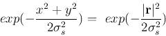
• A Gassion function (used before for modeling the center-surround RF of the retina ganglion cells) is used to model the spatially limited receptive field of a V1 cell:
  
  $$\mbox{ }exp(-\frac{x^2+y^2}{2\sigma_s^2}) = \mbox{ }exp(-\frac{ \vert {\bf r} \vert ^2}{2\sigma_s^2} )$$
  
  
  where ${\bf r}=[x, y]$ is a vector representing a position in the 2D visual space, $\sigma_s$ represents the size of the RF, and the subsript s is for space.

  

• A 2D sinusoidal function is used to model the V1 (simple) cells' receptive field of certain orientations:
  
  $$cos[(\omega_x x+\omega_y y)+\theta] =cos[( {\bf r} \cdot {\bf\omega}_s)+\theta]$$
  
  
  where $\omega_x$ and $\omega_y$ are the spatial frequencies in the x and y directions, respectively, ${\bf\omega}_s=[\omega_x, \omega_y]$ is a vector representing the spatial frequency, and $\theta$ is a phase angle which determines where in the elongated receptive field the $+$ and $-$ regions are (responding to bright and dark stimuli, respectively).

  

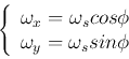
Note that the 2D spatial frequency vector ${\bf\omega}_s=[\omega_x, \omega_y]$ can be expressed by its magnitude $\omega_s$ and direction n (a unit vector along the direction):

$$\left\{ \begin{array}{l} \omega_s=\sqrt{\omega_x^2+\omega_y^2... ...=[cos \mbox{ } \phi, sin \mbox{ } \phi] \end{array} \right.$$

where $\phi=tan^{-1} (\omega_y/\omega_x)$, and equivalently the two spatial frequency components in $x$ and $y$ can be written as

$$\left\{ \begin{array}{l} \omega_x=\omega_s \mobx{ } cos \phi \\ \omega_y=\omega_s \mobx{ } sin \phi \end{array} \right.$$

The product of the above two functions is a Gabel function which is used to model the receptive field of a V1 cell:

$$G(x,y)=exp(-\frac{ \vert {\bf r} \vert ^2 }{2\sigma_s^2} ) \mbox{ } cos[( {\bf r} \cdot {\bf\omega}_s)+\theta]$$