Let A and B be two random events and P(A) and P(B) be their probabilities.
The probability of the joint event of both A and B, represented by P(A,B),
can be obtained as
If the two events are independent of each other, i.e., how likely event A will
occur is independent of whether event B occurs, and vice versa, then
The response property of a neuron can be characterized by the tuning curve which represents how the neuron responds differently to stimulus with a varying parameter. When there are two varying parameter, the tuning surface is used. The shape of one dimensional tuning curves usually fall into one of two categories, sigmoidal shaped, as the tuning for contrasts or near and far stereo cells for distances, and bell shaped (Gaussian), as for orientation or direction of motion.
The a neuron is treated as a communication channel which receives the stimuli
s(t) as the input and generates the spike trains
![]() as
the output. Here both s(t) and x(t) are treated as random variables and the
observing x(t) as the response to s(t) is considered as a process in which
certain information (e.g., about the external world from the sensory stimuli) is
gained. To describe the relationship between them, that is, how the stimulus affects
the response and how the response reflects the stimulus, we define
as
the output. Here both s(t) and x(t) are treated as random variables and the
observing x(t) as the response to s(t) is considered as a process in which
certain information (e.g., about the external world from the sensory stimuli) is
gained. To describe the relationship between them, that is, how the stimulus affects
the response and how the response reflects the stimulus, we define
These probabilities are all related to the joint probability of both s(t) and
x(t)
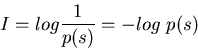
p(s) is also called the a priori probability of input s, as it represents
the likelihood of s before the neuron responding to it; and p(s/x) is called
the post priori probability of s, as it represents the likelihood of s
given that the neuron has responded to it by of x. As observing x will always
more or less gain some information about s, we have
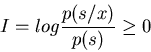
The total information gained from this process is quantitatively given by
In the ideal case without noise, complete information about the stimuli can be
obtained in the sense that any given stimulus s is responded to with a specific
x, i.e,, p(s/x)=1,
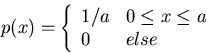
If the input is not a binary random event (either happens or not with probability
P), but a random variable of varying values s with probability distribution
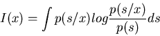
p(s), then the information gained in an ideal communication channel is the
weighted average of information for all possible values of s:
If the system is noisy, the stimulus-response relationship is no longer definite, as the same s may be responded to with different x due to noise, i.e., p(s/x) < 1. Here we first find the information about s gained when observing a particular x:
| I | = | 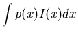 |
|
| = | ![$\displaystyle \int [ \int p(s/x) log \frac{p(s/x)}{p(s)} ds ] dx$](img39.gif) |
||
| = | ![$\displaystyle \int p(x) [ \int p(s/x) log p(s/x) ds ] dx -\int p(x) [\int p(s/x) log p(s) ds] dx$](img40.gif) |
||
| = | ![$\displaystyle \int p(x) [ \int p(s/x) log p(s/x) ds ] dx -\int [\int p(x) p(s/x) dx] log p(s) ds$](img41.gif) |
||
| = | H(s)-H(s/x) |
We define H(s) as the entropy of s. Note that as H(s) is the same as the complete information gained in the ideal case, it represents the maximum possible information available about s that can be gained. Since information gaining can be considered the same process as uncertainty reduction, H(s) also represents the uncertainty about s before observing x. And H(s/x) is the conditional entropy, representing the uncertainty of s after observing x. If the base of logarithm is 2, the unit of entropy is bit.
The information gained
I=H(s)-H(s/x) is thus called mutual information
and represents the uncertainty reduction from H(s) before observing x to
H(s/x) after observing x. In the ideal case p(s/x)=1, after observing s
the uncertainty becomes zero H(s/x)=0, and the complete information about s
![]() is gained.
is gained.
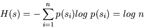
As an example, consider an experiment with n equally likely possible outcomes
si (
![]() ). The probability for a particular si to occur is
p(si)=1/n. Now the total uncertainty, the entropy, of this experiment is
). The probability for a particular si to occur is
p(si)=1/n. Now the total uncertainty, the entropy, of this experiment is
Here we find the probability distribution p(x) to maximize the entropy
![]() subject to some given conditions, as well as
subject to some given conditions, as well as
This kind of constrained optimization problem can be solved by Lagrange multiplier method.
Also as the variance ![]() can be considered as the dynamic energy contained
in x, we see that among all possible distributions with the same uncertainty,
Gaussian distribution requires the minimum energy.
can be considered as the dynamic energy contained
in x, we see that among all possible distributions with the same uncertainty,
Gaussian distribution requires the minimum energy.
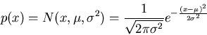
If the only knowledge about a random experiment is the mean ![]() and variance
and variance
![]() (which can be estimated by carrying the experiment a large number of
times), then its unknown probability distribution can be best estimated by a
normal distribution
(which can be estimated by carrying the experiment a large number of
times), then its unknown probability distribution can be best estimated by a
normal distribution
![]() ,
as it imposes minimum artificial
constraint by allowing the maximum uncertainty.
,
as it imposes minimum artificial
constraint by allowing the maximum uncertainty.
We now know that the amount of information available about the external world is limited by the entropy of the input sensory signals. And, on the other hand, how much information about the sensory input the spike trains can provide is limited by the entropy of these spike trains, as considered below.
Here we ignore the temporal pattern of the spike trains and characterize each
spike train only by the total number of spikes n in a time window T. The range
of n is
![]() .
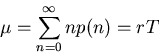
The mean of n is
.
The mean of n is
It can be shown that the distribution with maximum entropy is
To find the entropy per unit time, we divide H(n) by T to obtain the
entropy rate (bit per second) representing amount of information gained
per unit time. Or, to find the information carried by each spike, we divide
H(n) by ![]() .
.
Shown in the plot is the plot of entropy per spike as a function of ![]() .
.
To compute the entropy without ignoring the temporal pattern of the spike train,
we divide the time window T into ![]() bins of width
bins of width ![]() where
where ![]() is
short to allow no more than one spike to fit in (but long enough so that a spike
never needs to take two bins time). Now each spike train can be represented by a
N-bit string of 0's and 1's. The number of 1's in the string is N1=rT, where
r is the firing rate, number of spikes per unit time). And the probability for
any bit to be 1 is p=N1/N.
is
short to allow no more than one spike to fit in (but long enough so that a spike
never needs to take two bins time). Now each spike train can be represented by a
N-bit string of 0's and 1's. The number of 1's in the string is N1=rT, where
r is the firing rate, number of spikes per unit time). And the probability for
any bit to be 1 is p=N1/N.
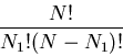
The total number of different equally likely patterns of the string is
(choosing N1 of N bins to be 1):
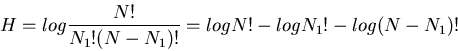
To deal with the factorials, use Stirling's formula
| H | = | -N [ log p +(1-p) log (1-p) ] | |
| = | ![$\displaystyle -\frac{T}{\tau}[(r\tau)log (r\tau) +(1-r\tau) log (1-r\tau)]$](img73.gif) |
Comparing this plot with that of the spike count entropy, we see that each spike now carry more information.
Let A and B be two random events and P(A) and P(B) be their probabilities.
The probability of the joint event of both A and B, represented by P(A,B),
can be obtained as
If the two events are independent of each other, i.e., how likely event A will
occur is independent of whether event B occurs, and vice versa, then
Stimuli and responses as random variables
The response property of a neuron can be characterized by the tuning curve which represents how the neuron responds differently to stimulus with a varying parameter. When there are two varying parameter, the tuning surface is used. The shape of one dimensional tuning curves usually fall into one of two categories, sigmoidal shaped, as the tuning for contrasts or near and far stereo cells for distances, and bell shaped (Gaussian), as for orientation or direction of motion.
The a neuron is treated as a communication channel which receives the stimuli
s(t) as the input and generates the spike trains
![]() as
the output. Here both s(t) and x(t) are treated as random variables and the
observing x(t) as the response to s(t) is considered as a process in which
certain information (e.g., about the external world from the sensory stimuli) is
gained. To describe the relationship between them, that is, how the stimulus affects
the response and how the response reflects the stimulus, we define
as
the output. Here both s(t) and x(t) are treated as random variables and the
observing x(t) as the response to s(t) is considered as a process in which
certain information (e.g., about the external world from the sensory stimuli) is
gained. To describe the relationship between them, that is, how the stimulus affects
the response and how the response reflects the stimulus, we define
These probabilities are all related to the joint probability of both s(t) and
x(t)
Neuronal response as communication channel
p(s) is also called the a priori probability of input s, as it represents
the likelihood of s before the neuron responding to it; and p(s/x) is called
the post priori probability of s, as it represents the likelihood of s
given that the neuron has responded to it by of x. As observing x will always
more or less gain some information about s, we have
The total information gained from this process is quantitatively given by
Information I - ideal case
In the ideal case without noise, complete information about the stimuli can be
obtained in the sense that any given stimulus s is responded to with a specific
x, i.e,, p(s/x)=1,
If the input is not a binary random event (either happens or not with probability
P), but a random variable of varying values s with probability distribution
p(s), then the information gained in an ideal communication channel is the
weighted average of information for all possible values of s:
Information II - with noise
If the system is noisy, the stimulus-response relationship is no longer definite, as the same s may be responded to with different x due to noise, i.e., p(s/x) < 1. Here we first find the information about s gained when observing a particular x:
| I | = | |
|
| = | |
||
| = | |
||
| = | |
||
| = | H(s)-H(s/x) |
Entropy
We define H(s) as the entropy of s. Note that as H(s) is the same as the complete information gained in the ideal case, it represents the maximum possible information available about s that can be gained. Since information gaining can be considered the same process as uncertainty reduction, H(s) also represents the uncertainty about s before observing x. And H(s/x) is the conditional entropy, representing the uncertainty of s after observing x. If the base of logarithm is 2, the unit of entropy is bit.
The information gained
I=H(s)-H(s/x) is thus called mutual information
and represents the uncertainty reduction from H(s) before observing x to
H(s/x) after observing x. In the ideal case p(s/x)=1, after observing s
the uncertainty becomes zero H(s/x)=0, and the complete information about s
![]() is gained.
is gained.
As an example, consider an experiment with n equally likely possible outcomes
si (
![]() ). The probability for a particular si to occur is
p(si)=1/n. Now the total uncertainty, the entropy, of this experiment is
). The probability for a particular si to occur is
p(si)=1/n. Now the total uncertainty, the entropy, of this experiment is
Entropy under given conditions
Here we find the probability distribution p(x) to maximize the entropy
![]() subject to some given conditions, as well as
subject to some given conditions, as well as
This kind of constrained optimization problem can be solved by Lagrange multiplier method.
Also as the variance ![]() can be considered as the dynamic energy contained
in x, we see that among all possible distributions with the same uncertainty,
Gaussian distribution requires the minimum energy.
can be considered as the dynamic energy contained
in x, we see that among all possible distributions with the same uncertainty,
Gaussian distribution requires the minimum energy.
If the only knowledge about a random experiment is the mean ![]() and variance
and variance
![]() (which can be estimated by carrying the experiment a large number of
times), then its unknown probability distribution can be best estimated by a
normal distribution
(which can be estimated by carrying the experiment a large number of
times), then its unknown probability distribution can be best estimated by a
normal distribution
![]() ,
as it imposes minimum artificial
constraint by allowing the maximum uncertainty.
,
as it imposes minimum artificial
constraint by allowing the maximum uncertainty.
Entropy of spike trains
We now know that the amount of information available about the external world is limited by the entropy of the input sensory signals. And, on the other hand, how much information about the sensory input the spike trains can provide is limited by the entropy of these spike trains, as considered below.
Here we ignore the temporal pattern of the spike trains and characterize each
spike train only by the total number of spikes n in a time window T. The range
of n is
![]() .
The mean of n is
.
The mean of n is
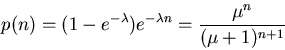
It can be shown that the distribution with maximum entropy is
To find the entropy per unit time, we divide H(n) by T to obtain the
entropy rate (bit per second) representing amount of information gained
per unit time. Or, to find the information carried by each spike, we divide
H(n) by ![]() .
.
Shown in the plot is the plot of entropy per spike as a function of ![]() .
.
To compute the entropy without ignoring the temporal pattern of the spike train,
we divide the time window T into ![]() bins of width
bins of width ![]() where
where ![]() is
short to allow no more than one spike to fit in (but long enough so that a spike
never needs to take two bins time). Now each spike train can be represented by a
N-bit string of 0's and 1's. The number of 1's in the string is N1=rT, where
r is the firing rate, number of spikes per unit time). And the probability for
any bit to be 1 is p=N1/N.
is
short to allow no more than one spike to fit in (but long enough so that a spike
never needs to take two bins time). Now each spike train can be represented by a
N-bit string of 0's and 1's. The number of 1's in the string is N1=rT, where
r is the firing rate, number of spikes per unit time). And the probability for
any bit to be 1 is p=N1/N.
The total number of different equally likely patterns of the string is
(choosing N1 of N bins to be 1):
To deal with the factorials, use Stirling's formula
| H | = | -N [ log p +(1-p) log (1-p) ] | |
| = | |
Comparing this plot with that of the spike count entropy, we see that each spike now carry more information.