next up previous
Next: Modeling a Spiking Neuron Up: No Title Previous: The Membrane Equation and

Measuring Neuronal Response - the Firing Rate

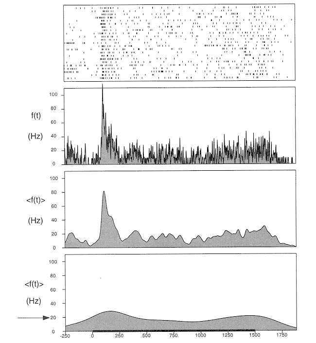
Neurons respond to external stimuli by generating a train of impulses (spikes) of action potentials. In a typical physiological experiment, the same stimulus is presented multiple times to a neuron and its response recorded (e.g., of 2 second long), as shown in the figure. The detailed compositions of the spike trains vary from trial to trial. To characterize the response of the neuron to the same stimulus, the average firing rate <f(t)> is computed by averaging the responses of all trials over a brief time window $\Delta T$ of a few msce. However, if the average time is too long, some details in the neuronal signal may be averaged out and thereby some useful information may be lost.

To model the spike trains of the neuronal response, we first treat each spike as a delta function:

\begin{displaymath}\delta(t)=\lim_{a \rightarrow \infty} \left\{ \begin{array}{l...
... \begin{array}{ll} \infty & t=0 \\ 0 & else \end{array}\right.
\end{displaymath}

Note that although the value of $\delta(t)$ is infinitely large at t=0, the area underneath the function (representing energy contained in the function) is finite (unit):

\begin{displaymath}\int_{-\infty}^{\infty} \delta(t) dt = 1 \end{displaymath}

A spike occurs at t=to is represented by $\delta(t-t_o)$. Now a train of spikes in the jth trial can be represented as

\begin{displaymath}T_j(t)=\sum_{i=1}^{n_j} \delta(t-t_{ij}) \end{displaymath}

where nj is the total number of spikes in the jth trial. If the experiment is repeated k times, the firing rate at time t is computed as the average over all k trials and over a time window of width $\Delta T$:
<f(t)> = $\displaystyle \frac{1}{k} \sum_{j=1}^k \frac{1}{\Delta T} \int_t^{t+\Delta T} T_j(\tau) d\tau$  
  = $\displaystyle \frac{1}{k} \sum_{j=1}^k \frac{1}{\Delta T} \int_t^{t+\Delta T}
\sum_{i=1}^{n_j} \delta(\tau-t_{ij}) d\tau$  

Alternatively, we can make the average more smooth over time by using a Gaussian function

\begin{displaymath}G(t,\sigma)=\frac{1}{\sqrt{2\pi \sigma^2}} e^{-\frac{t^2}{2\sigma^2}} \end{displaymath}

instead of a constant time window, as the weighting function. Note that $G(t,\sigma)$ also contains unit energy:

\begin{displaymath}\int_{-\infty}^{\infty} G(t, \sigma) dt = 1 \end{displaymath}

Now the smoothed firing rate as a function of time becomes
<f(t)> = $\displaystyle \frac{1}{k} \sum_{j=1}^k \frac{1}{\sqrt{2\pi \sigma^2}}
\int_{-\i...
...y} e^{-\frac{(t-\tau)^2}{2\sigma^2}}
\sum_{i=1}^{n_j} \delta(\tau-t_{ij}) d\tau$  

The resulting smoothed average firing rate is called post-stimulus time histogram (PSTH).

../figures/firingrate.gif


next up previous
Next: Modeling a Spiking Neuron Up: No Title Previous: The Membrane Equation and
Ruye Wang
1999-09-20