Modeling RF of Retina Cells II - Spatial Frequency Domain

Based on the spatial model of the RF

$$f(x,y)=k_c\mbox{ }exp[-\frac{x^2+y^2}{\sigma_c^2}] -k_s\mbox{ }exp[-\frac{x^2+y^2}{\sigma_s^2}]$$

we consider how this cell responds to gratings (spatial sinusoidal signals) of different frequencies. For simplicity, we reduce the spatial dimension from 2 to 1 to have the RF function as

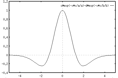
$$f(x)=k_c\mbox{ }exp[-\frac{x^2}{\sigma_c^2}] -k_s\mbox{ }exp[-\frac{x^2}{\sigma_s^2}]$$

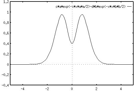
The Fourier transform of this function is

$$F(\omega)=k_c \sqrt{\pi \sigma_c^2}\mbox{ }exp[-(\frac{\omega... ...t{\pi \sigma_s^2}\mbox{ }exp[-(\frac{\omega \sigma_s^2}{2})^2]$$

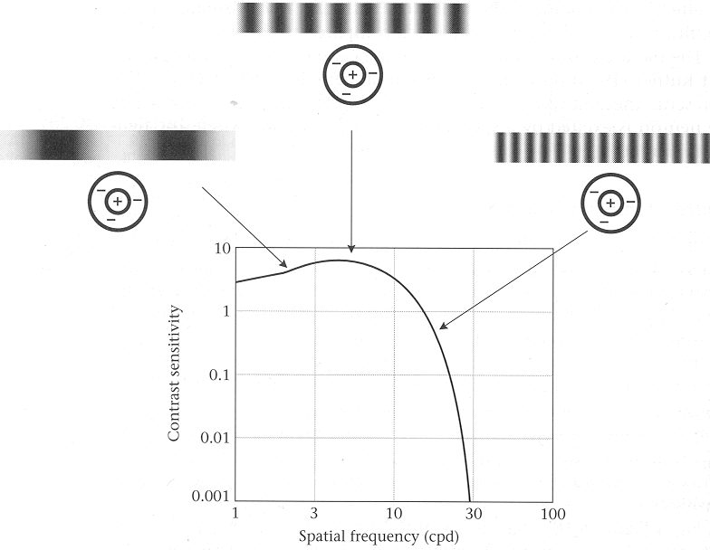
From the plot of the Fourier transform of the RF function we see that the cell will respond most strongly to gratings of a certain optimal frequency, but poorly to gratings of either higher or lower frequencies. In other words, the cell will behave like a band-pass filter. This can be explained in the following figure:

Note that the contributions from the center and surround of the RF cancel each other to cause a weak response when the spatial frequency is either too low or too high, but they add up cause a strong response when the frequency is about optimal.

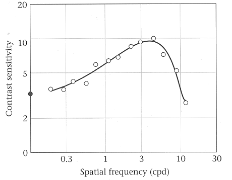
This filtering effect of the RF is confirmed by physiological studies, such as the frequency response of a monkey LGN cell by Derrington and Lennie (1984), as shown in this figure:

(In the two figures above, k_c=2, k_s=1, $\sigma_c=1.2$, $\sigma_s=2$.)