Modeling RF of Retina Cells I - Spatial Domain

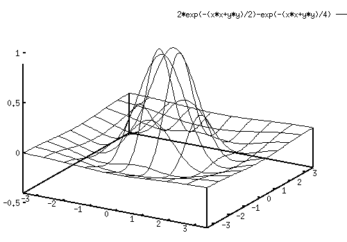
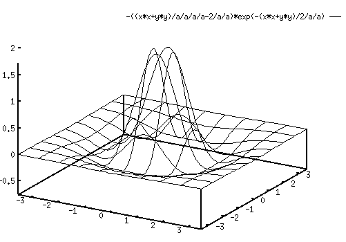
First we consider modeling the RF in the Space Domain. The center-surround RFs of the retina ganglion cells can be mathematically modeled in either of the following ways, both starts with 2D Caussian function defined as

$$G(x,y)=c\mbox{ }exp[-\frac{x^2+y^2}{2\sigma_c^2}]$$

which peaks at the origion and the parameter $\sigma$ determines how sharp the peak is. If G(x,y) is a Gassian probability density distribution of some two random variables x and y, then $\sigma$ represents the standard deviation of the distribution, and c is a normalizing coefficient so chosen that $\int \int G(x,y) dx dy = 1$.

• The first model is the sum of two 2D Gaussian functions of different hights (k_c, k_s), standard deviations ($\sigma_c$, $\sigma_s$), and opposite polarities:

  
  

  f₁(x,y) = G_center(x,y)-G_surround(x,y)

  $$k_c\mbox{ }exp[-\frac{x^2+y^2}{\sigma_c^2}]- k_s\mbox{ }exp[-\frac{x^2+y^2}{\sigma_s^2}]$$ =

  
  

  

• The second model is a function obtained by taking a Laplassian operation on a Gaussian function $G(x,y)=exp(-(x^2+y^2)/2\sigma^2)$. In general, the Laplassian operation of a two-variable function g(x,y) is defined as $\triangle g(x,y)\stackrel{\triangle}{=} \partial^2 g(x,y)/\partial x^2-\partial^2 g(x,y)/\partial y^2$.

  
  

  $$-\triangle G(x,y)$$ f₂(x,y) =

  $$-\frac{\partial^2 G(x,y)}{\partial x^2}- \frac{\partial^2 G(x,y)}{\partial y^2}$$ =

  $$[\frac{x^2+y^2}{\sigma^4}-\frac{2}{\sigma^2}] exp[-\frac{x^2+y^2}{2\sigma^2}]$$ =

  
  

  

This 2D function is someitmes called the impulse response function of the cell, although with a little different definition. (Impulse response funciton is usually defined as the time or spatial invariant response to an impulse.)

With certain simplifications, the cells can be assumed as linear systems. And a cell's response to a 2D stimulus (an image) s(x,y) located at a spatial position (0, 0) can be found as the weighted sum (integral):

$$r=\int \int_{-\infty}^{\infty} f(x,y) s(x,y) dx dy$$

The same 2D stimulus s(x,y) located at a different spatial position (say, by shifting) (u,v) can be represented by s(x-u, y-v), and the response to this stimulus becomes a function of the spatial location of the stimulus:

$$r(u,v)= \int \int_{-\infty}^{\infty} f(x,y) s(x-u,y-v) dx dy =\int \int_{-\infty}^{\infty} s(x,y) f(x-u,y-v) dx dy$$

This is the correlation of the stimulus s(x,y) and the RF function. But as the RF is central symmetric, i.e., f(x,y)=f(-x,-y), the correlation above can be written as the convolution of the stimulus s and the RF response f:

$$r(u,v)= \int \int_{-\infty}^{\infty} s(x,y) f(u-x,v-y) dx dy=s(u,v)*f(u,v)$$