The Walsh-Hadamard Transform (Hadamard Ordered)

As any orthogonal (unitary) matrix can be used to define a discrete orthogonal (unitary) transform, we define a Walsh-Hadamard transform of Hadamard order ($WHT_h$) as

$$\left\{ \begin{array}{l} {\bf X}={\bf H}{\bf x}\;\;\;\;\;\;\... ... x}={\bf H}{\bf X}\;\;\;\;\;\;\;(inverse) \end{array} \right.$$

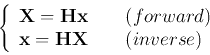
These are the forward and inverse $WHT_h$ transform pair. Note that the forward and inverse transforms are identical!

Here ${\bf x}=[ x[0], x[1], \cdots, x[N-1] ]^T$ and ${\bf X}=[ X[0], X[1], \cdots, X[N-1] ]^T$ are the signal and spectrum vectors, respectively. The $k$th element of the transform can also be written as

$$X[k]=\sum_{m=0}^{N-1}h[k,m] x[m] =\sum_{m=0}^{N-1}x[m] \prod_{i=0}^{n-1}(-1)^{m_ik_i}$$

The complexity of WHT is $O(N^2)$. Similar to FFT algorithm, we can derive a fast WHT algorithm with complexity of $O(N log_2 N)$. We will assume $n=3$ and $N=2^n=8$ in the following derivation. An $N=8$ point $WHT_h$ of signal $x[m]$ is defined as

$${\bf X}= \left[ \begin{array}{c} X[0] \vdots X[3] X... ... \vdots x[3] x[4] \vdots x[7] \end{array} \right]$$

Here for simplicity, we ignored the coefficient $1/\sqrt{2}$. This equation can be separated into two parts. The first half of the $X$ vector can be obtained as

$$\left[ \begin{array}{c} X[0] X[1] X[2] X[3] \end{ar... ...ay}{c} x_1[0] x_1[1] x_1[2] x_1[3] \end{array}\right]$$ (1)

where

$$x_1[i] \stackrel{\triangle}{=}x[i]+x[i+4] \;\;\;\;(i=0, \cdots ,3)$$ (2)

The second half of the $X$ vector can be obtained as

$$\left[ \begin{array}{c} X[4] X[5] X[6] X[7] \end{ar... ...ay}{c} x_1[4] x_1[5] x_1[6] x_1[7] \end{array}\right]$$ (3)

where

$$x_1[i+4] \stackrel{\triangle}{=}x[i]-x[i+4] \;\;\;\;(i=0, \cdots ,3)$$ (4)

What we have done is converting a $WHT$ of size $N=8$ into two $WHTs$ of size $N/2=4$. Continuing this process recursively, we can rewrite Eq. (1) as the following (similar process for Eq. (3))

$$\left[ \begin{array}{c} X[0] X[1] X[2] X[3] \end{ar... ...{c} x_1[0] x_1[1] x_1[2] x_1[3] \end{array} \right]$$

This equation can again be separated into two halves. The first half is

$$\left[ \begin{array}{c} X[0] X[1] \end{array} \right] ={\... ...{array}{c} x_2[0]+x_2[1] x_2[0]-x_2[1] \end{array} \right]$$ (5)

where

$$x_2[i] \stackrel{\triangle}{=}x_1[i]+x_1[i+2]\;\;\;\;(i=0,1)$$ (6)

The second half is

$$\left[ \begin{array}{c} X[2] X[3] \end{array} \right] ={\... ...{array}{c} x_2[2]+x_2[3] x_2[2]-x_2[3] \end{array} \right]$$ (7)

where

$$x_2[i+2] \stackrel{\triangle}{=}x_1[i]-x_1[i+2]\;\;\;\;(i=0,1)$$ (8)

$X[4]$ through $X[7]$ of the second half can be obtained similarly.

$$X[0]=x_2[0]+x_2[1]$$ (9)

and

$$X[1]=x_2[0]-x_2[1]$$ (10)

Summarizing the above steps of Equations (2), (4), (6), (8), (9) and (10), we get the Fast WHT algorithm as illustrated below.