Hadamard Matrix

The Kronecker product of two matrices ${\bf A}=[a_{ij}]_{m\times n}$ and ${\bf B}=[b_{ij}]_{k\times l}$ is defined as

$${\bf A} \otimes {\bf B} \stackrel{\triangle}{=}\left[ \begin{... ...B} & \cdots & a_{mn}{\bf B} \end{array} \right]_{mk \times nl}$$

In general, ${\bf A}\otimes {\bf B} \neq {\bf B}\otimes {\bf A}$.

The Hadamard Matrix is defined recursively as below:

$${\bf H}_1 \stackrel{\triangle}{=} \frac{1}{\sqrt{2}} \left[ \begin{array}{rr} 1 & 1 1 & -1 \end{array} \right]$$

$${\bf H}_n={\bf H}_1\otimes{\bf H}_{n-1}=\frac{1}{\sqrt{2}}\... ...}_{n-1} {\bf H}_{n-1} & -{\bf H}_{n-1} \end{array} \right]$$

Obviously ${\bf H}^T={\bf H}$ is rean and symmetric. Here are two examples for $n=2$ and $n=3$:

$${\bf H}_2={\bf H}_1 \otimes {\bf H}_1=\frac{1}{\sqrt{2}}\left... ... 1 & 1 & -1 & -1 1 & -1 & -1 & 1 \\ \end{array} \right]$$

$${\bf H}_3={\bf H}_1 \otimes {\bf H}_2=\frac{1}{\sqrt{2}}\left... ... 3 3 & 4 \\ 4 & 1 5 & 6 6 & 2 7 & 5 \end{array}$$

Note that ${\bf H}_n$ is $N=2^n$ by $N=2^n$ matrix.

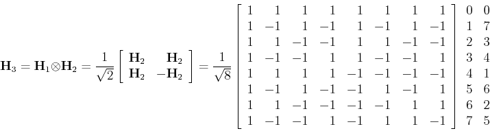
The first column on the right of the matrix ${\bf H}_3$ is for the indecies of the $N=8$ rows, and the second column represents the sequency (the number of zero-crossings or sign changes) in each row. Sequency is similar to but different from frequency in the sense that it measures the rate of change of non-periodical signals.

The rows of the matrix can be considered as the $N=2^3$ samples of the following waveforms:

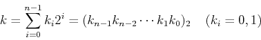
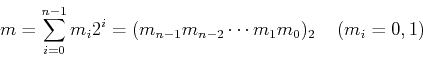
The Hadamard matrix can also be obtained by defining its element in the kth row and mth column of $H$ as

$$h[k,m]=(-1)^{\sum_{i=0}^{n-1}k_im_i} =\prod_{i=0}^{n-1} (-1)^{k_im_i}=h[m,k] \;\;\;\;\; (k,m=0,1,\cdots,N-1)$$

where

$$k=\sum_{i=0}^{n-1}k_i2^i=(k_{n-1}k_{n-2}\cdots k_1k_0)_2 \;\;\;\;(k_i=0,1)$$

$$m=\sum_{i=0}^{n-1}m_i2^i=(m_{n-1}m_{n-2}\cdots m_1m_0)_2 \;\;\;\;(m_i=0,1)$$

i.e., $(k_{n-1}k_{n-2}\cdots k_1k_0)_2$ and $(m_{n-1}m_{n-2}\cdots m_1m_0)_2$ are the binary representations of $k$ and $m$, respectively. Obviously, $n=log_2 N$.

We can show the Hadamard matrix ${\bf H}$ is orthogonal by induction. First, it is obvious that ${\bf H}_1$ is orthogonal:

$${\bf H}_1^T{\bf H}_1={\bf H}_1{\bf H}_1 =\frac{1}{2}\left[... ...egin{array}{rr}1&0 0&1\end{array}\right]={\bf I}_{2\times 2}$$

Next we assume ${\bf H}_{n-1}$ is orthogonal, i.e.,

$${\bf H}^T_{n-1}{\bf H}_{n-1}={\bf H}_{n-1}{\bf H}_{n-1}={\bf I}_{2^{n-1}\times 2^{n-1}}$$

Finally we show that ${\bf H}_n={\bf H}_1\otimes{\bf H}_{n-1}$ is also orthogonal:

$${\bf H}_n^T{\bf H}_n={\bf H}_n{\bf H}_n = \frac{1}{2}\left[ \begin{array}{rr} {\bf H}_{n-1} & {\bf H}_{n-... ...f H}_{n-1} & {\bf H}_{n-1} {\bf H}_{n-1}&-{\bf H}_{n-1} \end{array} \right]$$

$$= \frac{1}{2}\left[\begin{array}{rr}{\bf H}_{n-1}{\bf H}_{n-1}+{\bf... ...\bf H}_{n-1}+{\bf H}_{n-1}{\bf H}_{n-1}\end{array}\right] ={\bf I}_{N\times N}$$

In summary, the Hadamard matrix ${\bf H}$ is real, symmetric, and orthogonal:

$${\bf H}={\bf H}^*={\bf H}^T={\bf H}^{-1}$$