Wavelet Expansion

For a specific value $j=j_0$, the equation discussed above can be written as

$$L^2(R)=V_{\infty}=V_{j_0} \oplus W_{j_0} \oplus W_{j_0+1} \oplus W_{j_0+2} \oplus \cdots$$

which indicates that any square-integrable function $x(t) \in L^2$ can be expanded as a linear combination of both the scaling basis functions $\varphi_{j_0,k}(t)$ and the wavelet basis functions $\psi_{j,k}(t)$ ( $j=j_0, j_0+1,\cdots$):

$$x(t)=\sum_k c_{j_0,k}\varphi_{j_0,k}(t)+\sum_{j=j_0}^{\infty} \sum_k d_{j,k}\psi_{j,k}(t)$$

where $c_{j_0,k}$ is the approximation coefficient:

$$c_{j_0,k}=(x(t),\varphi_{j_0,k}(t))=\int x(t)\varphi_{j_0,k}(t) dt$$

and $d_{j,k}$ is the detail coefficient:

$$d_{j,k}=(x(t),\psi_{j,k}(t))=\int x(t)\psi_{j,k}(t) dt$$

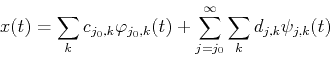
The first term contained in the wavelet expansion of the function $x(t)$ represents the approximation of the function at scale level $j_0$ by the linear combination of the scaling functions $\varphi_{j_0,k}(t)$, and the summation with index $j$ in the second term in the expansion is for the details of different levels contained in the function $x(t)$ approximated by the linear combination of the wavelet functions of progressively higher scales $j_0+1, j_0+2, \cdots$.

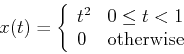
An Example

A continuous function $x(t)$ is defined over the period $0 \le t < 1$ as:

$$x(t)=\left\{ \begin{array}{ll} t^2 & 0\le t < 1 0 & \mbox{otherwise} \end{array} \right.$$

We use Haar wavelets, and a starting scale $j_0=0$. Each individual space ($V_0$, $W_0$, $W_1$, $\cdots$) is spanned by different number of basis functions. For example, there is only one basis function in spaces $V_0$ and $W_0$, while space $W_1$ is spanned by 2 bases, and space $W_2$ is spanned by 4 bases (See Haar matrix).

$$c_0(0)=\int_0^1 t^2 \varphi_{0,0}(t) dt=\int_0^1 t^2 (t) dt=\frac{1}{3}$$

$$d_0(0)=\int_0^1 t^2 \psi_{0,0}(t) dt =\int_0^{0.5} t^2 (t) dt-\int_{0.5}^1 t^2 (t) dt=-\frac{1}{4}$$

$$d_1(0)=\int_0^1 t^2 \psi_{1,0}(t) dt =\int_0^{0.25} \sqrt{2}... ...dt-\int_{0.25}^{0.5} t^2 \sqrt{2}(t) dt =-\frac{\sqrt{2}}{32}$$

$$d_1(1)=\int_0^1 t^2 \psi_{1,1}(t) dt =\int_{0.5}^{0.75} \sqr... ...t) dt-\int_{0.75}^1 t^2 \sqrt{2}(t) dt =-\frac{3\sqrt{2}}{32}$$

Therefore the wavelet series expansion of the function $x(t)$ is

$$x(t)=\frac{1}{3}\varphi_{0,0}(t)+[-\frac{1}{4}\psi_{0,0}(t)] ... ...}{32}\psi_{1,0}(t)-\frac{3\sqrt{2}}{32}\psi_{1,1}(t)]+ \cdots$$

Here the first term is $V_0$, the second term is $W_0$, the third term is $W_1$, and $V_1=V_0 \oplus W_0$, $V_2=V_1\oplus W_1=V_0\oplus W_0 \oplus W_1$

This process can be carried out further. By contineously reducing the scale by half (spaces $V_3, V_4, \cdots$), higher temporal resolution (always doubled) is achieved. However, at the same time, the frequency resolution is reduced (always halved), as shown in the Heisenberg box.