Next: About this document ...
Up: svd
Previous: Conservation of Degrees of
SVD image transform has different applications in image processing and
analysis. We now consider how it can be used for data compression.
First we write a matrix  as
as
where
![${\bf a}_i=[a(1,i),\cdots,a(N,i)]^T$](img48.png) is the ith column vector of
is the ith column vector of  .
The total amount of energy contained in can be represented by the
norm of defined as
.
The total amount of energy contained in can be represented by the
norm of defined as
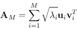
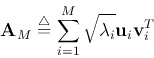
Now we consider image compression achieved by using only the first  eigenimages of the given image :
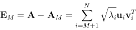
with error
After compression, the energy (information) contained in  is:
is:
Note that here we have used the property that
 .
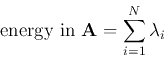
We see that the total amount of energy (information) contained in the
original image is
.
We see that the total amount of energy (information) contained in the
original image is
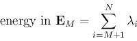
and the energy (information) lost (contained in  ) is
) is
It is therefore obvious that minimum energy is lost if we range
 's so that
To find out the compression ratio, consider total degrees of freedom in
:
The degrees of freedom in the  orthogonal vectors
 are
are
The same is true for
 . Including the
degrees of freedom in
. Including the
degrees of freedom in
 , we have the total d.o.f.:
and the compression ratio is
For example,  ,
,  , the compression rate is less than
  .
.
An example of using SVD for image compression is available
here
Next: About this document ...
Up: svd
Previous: Conservation of Degrees of
Ruye Wang
2014-08-20
![$\displaystyle {\cal E}_A=\parallel {\bf A} \parallel \stackrel{\triangle}{=} tr\;[{\bf A}^T{\bf A}]$](img49.png)
![$\displaystyle tr \left[ \begin{array}{c} {\bf a}_1^T \vdots {\bf a}_N^T...
...ts {\bf a}^T_N{\bf a}_1 & \cdots & {\bf a}_N^T{\bf a}_N
\end{array} \right]$](img51.png)
![$\displaystyle tr \; [{\bf A}_M^T{\bf A}_M]=
tr \left[ \sum_{i=1}^M\sqrt{\lamb...
...u}_i^T \right]
\left[ \sum_{j=1}^M\sqrt{\lambda_j}{\bf u}_j{\bf v}_j^T \right]$](img58.png)
![$\displaystyle tr \left[\sum_{i=1}^M (\sum_{j=1}^M\sqrt{\lambda_i}\sqrt{\lambda_...
...}_j^T ) \right]
= tr \left[\sum_{i=1}^M \lambda_i {\bf v}_i{\bf v}_i^T \right]$](img59.png)
![$\displaystyle \sum_{i=1}^M \lambda_i tr\; [{\bf v}_i{\bf v}_i^T ]
=\sum_{i=1}^M \lambda_i {\bf v}_i^T{\bf v}_i =\sum_{i=1}^M \lambda_i$](img60.png)