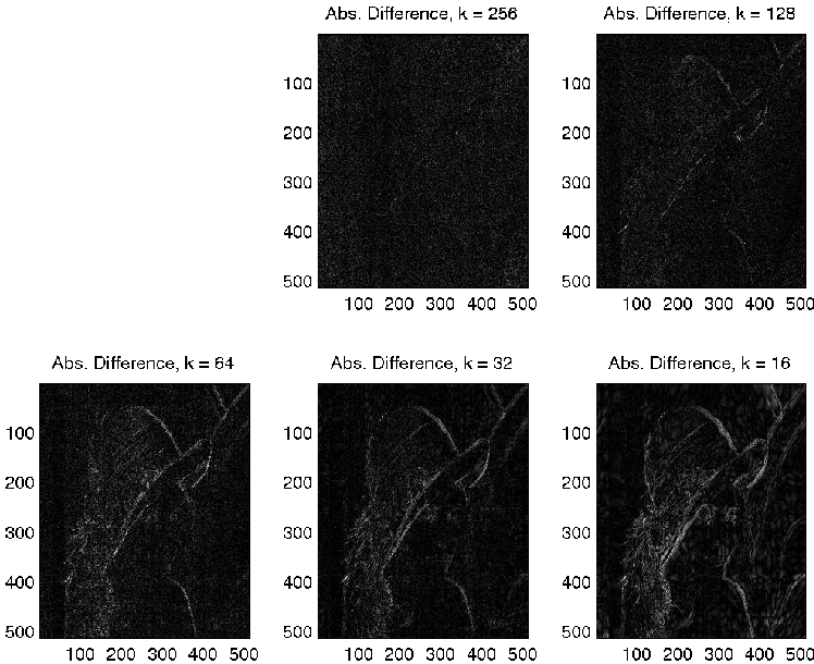
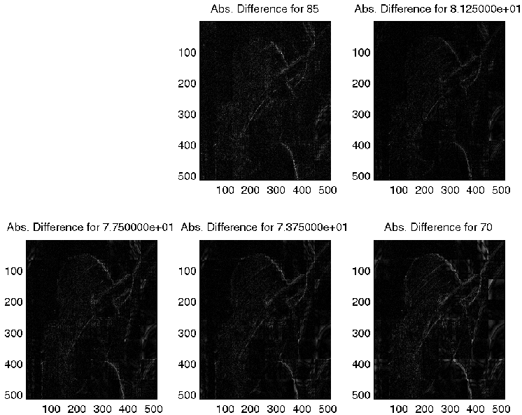
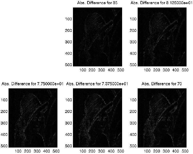
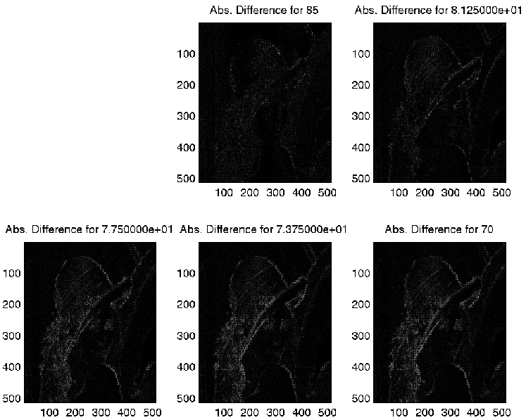
Figure 2. The absolute difference between the original and the re-constructed images.
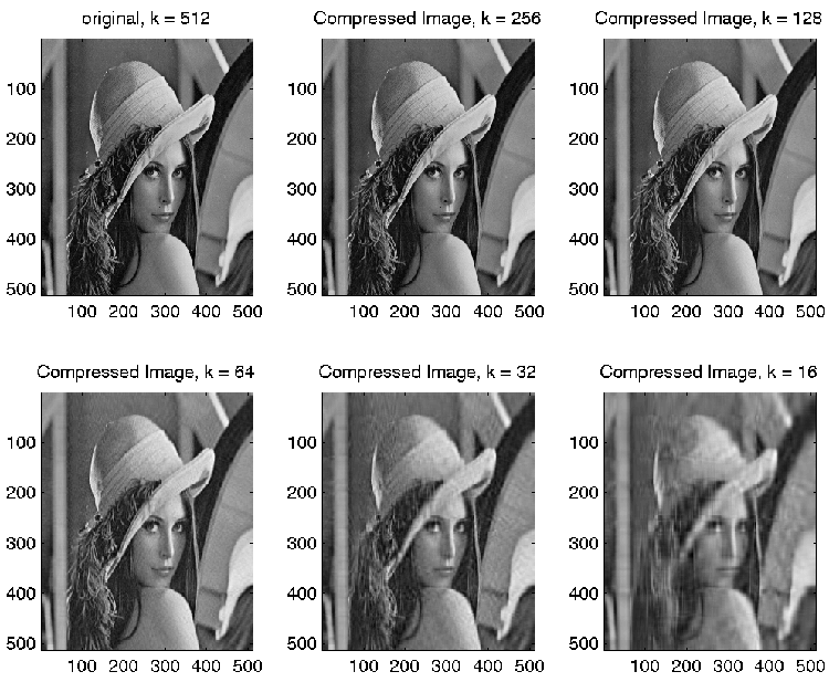
Original Image: 	A = USVH,
			where U is m by n,
			      V is n by n,
			      and S =
			      diag(r1, r2,...,rk,0,...,0)

Re-constructed Image:  A1 = US1VH,
			where U is m by k1,
			      V is k1 by n,
			      and S1 =
			      diag(r1, r2,...,rk1)

			and
		        ||A - A1||2 = rk1 + 1
PSNR = 10 log10((max. range)2 / Root Mean Square Error )
Rank k1 used for each sub-block:
					(r1+r2+...+rk1)
		Specified Percentage =------------------
					(r1+r2+...+rk)
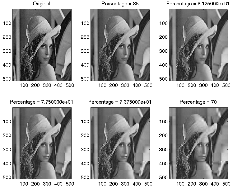
	Ranks used for percentage = 7.750000e+01:


	RUsed =

     1     5     2     4     3     1     3     8
     2     7    10     8     4     5     6     7
     1     5    12    10     6     5     7     2
     1     6    11    13     5     8     5     1
     2    12    15    11     4     8     3     2
     2    14    13     9     5     8     1     1
     3    14    13    11     2     6     3     4
     3    15    15     6     1     3     4     7


	Ranks used for percentage = 70:

	RUsed =

     1     1     1     2     2     1     2     5
     1     2     5     4     3     3     4     5
     1     3     7     6     3     3     5     1
     1     3     8     9     3     5     3     1
     1     9    12     8     3     5     2     1
     1    10    10     5     3     5     1     1
     2    11    10     6     1     4     2     3
     2    10    12     4     1     2     3     5
64-by-64 block-size:
===>    Percentage of Singular     |    Average Ranks   | Avg. Percentage of
        Values Sum                         Used           Ranks Used.
                85                      10.500000          0.164062
                81.25                   7.968750           0.124512
                77.5                    6.156250           0.096191
                73.75                   4.937500           0.077148
                70                      4.046875           0.063232


8-by-8 block-size:
===>    Percentage of Singular     |    Average Ranks   | Avg. Percentage of
        Values Sum                         Used           Ranks Used.
                85                      1.540039           0.192505
                81.25                   1.371582           0.171448
                77.5                    1.256104           0.157013
                73.75                   1.176514           0.147064
                70                      1.115234           0.139404
Original Image: 	A - mean = USVH,
			where U is m by n,
			      V is n by n,
			      and S =
			      diag(r1, r2,...,rk,0,...,0)

Re-constructed Image:  A1 = US1VH + mean,
			where U is m by k1,
			      V is k1 by n,
			      and S1 =
			      diag(r1, r2,...,rk1)
8-by-8 block-size:
===>    Percentage of Singular     |    Average Ranks   | Avg. Percentage of
        Values Sum                         Used           Ranks Used.
                85                      2.311279           0.288910
                81.25                   1.371582           0.171448
                77.5                    1.015137           0.126892
                73.75                   1.000000           0.125000
                70                      1.000000           0.125000

m = 0.3884       <---- mean
% function SDVCompression_3(F, BlockSize, SP, EP)
% Image Compression, take out the mean
%
%
% F: input file, a 2-D array
% BlockSize: 64, 32, 16, 8
% SP: Staring percentage of singular values AREA used
% EP: Ending percentage of singular values AREA used
% SP < EP
%
%
% testing my idea of using cumulative singularvalues
%
% James Chen, 11/30/2000
% ECS 289K, Project
%
close all
if (SP > EP)
disp('SP must be smaller than EP!!!')
return
end
% read in the image
IMG1 = imread(F);
X1org = im2double(IMG1);
XSize = size(X1org);
figure(1);
colormap(gray);
imagesc(X1org);
title (sprintf('Original Image: %s, Size: %i x %i', F, XSize(1), XSize(2)));
% mean
m = mean(mean(X1org))
X1org = X1org - m;
% display the image
figure(2);
subplot(2,3,1);
% shown in original size: imshow(X1org);
% or: in matrix format:
colormap(gray);
imagesc(X1org+m);
%title ('Original');
NumBlocks = XSize(1)/BlockSize;
PercentageStep = (EP - SP)/4.0;
Percentage = EP;
pl = 2;
while (pl <= 6)
for i = 1:NumBlocks
r = (i-1) * BlockSize + 1;
for j = 1:NumBlocks
%disp(sprintf('Processing block %i %i', i,j))
c = (j-1) * BlockSize + 1;
TB = X1org(r:r+BlockSize-1, c: c+BlockSize-1);
[TU,TS,TV] = svd(TB);
%U(i, j, :, :) = TU;
%S(i, j, :, :) = TS;
%V(i, j, :, :) = TV;
SV = diag(TS); % a n by 1 vector
% cumulative sum of singular values
s = size(SV);
R(i,j) = s(1);
% rank for original block
TCS(1) = SV(1);
for k = 2: s(1)
TCS(k) = TCS(k-1) + SV(k);
end
%CS(i,j,:,:) = TCS;
%
% reconstruction, de-compression
%
v = TCS(s(1)) * Percentage *0.01;
% find the rank used for each block
rr = 1;
k = s(1)-1;
while (k >=1)
if ( (TCS(k) <= v) & (TCS(k+1) >= v))
rr = k+1;
break;
end;
k = k-1;
end
RUsed(i,j) = rr;
PRUsed(i,j) = rr/s(1);
%disp(sprintf('rank used = %i', rr))
X = TU(:, 1:rr) * TS(1:rr, 1:rr) * TV(:, 1:rr)';
CI(r:r+BlockSize-1, c: c+BlockSize-1) = X;
end
end
% add the mean back to image
CI = CI + m;
disp('--------------')
disp(sprintf('Rnaks used for percentage = %i:\n', Percentage))
RUsed
avg = sum(sum(RUsed))/(NumBlocks*NumBlocks);
disp(sprintf('Average ranks used = %f\n\n', avg))
disp(sprintf('Ranks used / %i:', s(1)))
PRUsed
avg = sum(sum(PRUsed))/(NumBlocks*NumBlocks);
disp(sprintf('Average percentage of ranks used = %f\n', avg))
%display
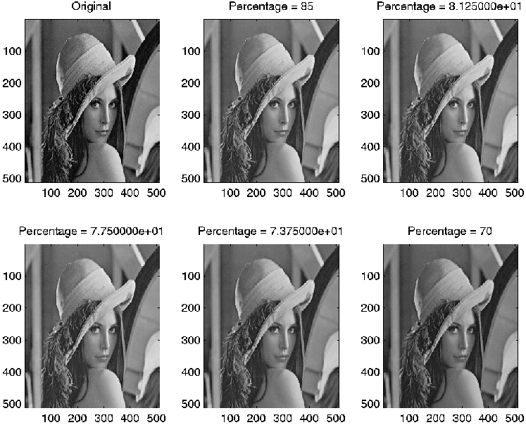
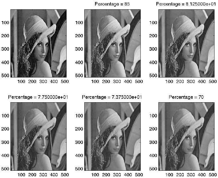
figure(2)
subplot(2,3, pl);
colormap(gray);
imagesc(CI);
title(sprintf('Percentage = %i', Percentage))
% !!!! add th emean back to the original picture
X1org = X1org + m;
Diff = X1org - CI;
figure(3)
subplot(2,3, pl);
colormap(gray);
imagesc(Diff);
title(sprintf('Difference for %i', Percentage))
figure(4)
subplot(2,3, pl);
colormap(gray);
imagesc(abs(Diff));
title(sprintf('Abs. Difference for %i', Percentage))
%figure(5)
%subplot(2,3,pl)
%bar(RUsed)
%title('Ranks used for each sub-block');
%axis([0 NumBlocks+1 0 s(1)]);
%figure(6)
%subplot(2,3,pl)
%bar(PRUsed)
%title('Percentage of the ranks used');
%axis([0 NumBlocks+1 0 1]);
Percentage = Percentage - PercentageStep;
pl = pl + 1;
% compute Peak SN ratio:
mse1 = 0;
for i = 1: XSize(1)
for j = 1: XSize(2)
mse1 = mse1 + Diff(i,j)*Diff(i,j);
end
end
mse1 = mse1 /(XSize(1) * XSize(2));
mse1 = sqrt(mse1)
PSNR = 10 * log10(255^2/mse1)
end