Next: Application in Image Compression
Up: svd
Previous: SVD Transform
We now show that the degrees of freedom (d.o.f., the number of independent
variables in the signal) are conserved in the SVD transform (same as any other
transforms). In spatial domain the d.o.f. of the image matrix
 (assuming
  for simplicity) is
  . Now in the transform domain,
both
. Now in the transform domain,
both  and
and  have the same d.o.f.
  for the following
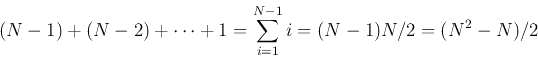
reason. The first column vector has
for the following
reason. The first column vector has  elements subject to normalization, i.e.,
 d.o.f.; the second vector is the same except it also has to be orthogonal
to the first one, and therefore has
d.o.f.; the second vector is the same except it also has to be orthogonal
to the first one, and therefore has  d.o.f.; the third vector has to be
orthogonal to the first two vectors and therefore has
d.o.f.; the third vector has to be
orthogonal to the first two vectors and therefore has  d.o.f.; etc. Now
the total d.o.f. of all vectors is
d.o.f.; etc. Now
the total d.o.f. of all vectors is
Together with the d.o.f. in  , the over all d.o.f. is
This indicates that the signal, in either the original spatial domain ( ) or
the transform domain (,
) or
the transform domain (,  and
and  ), always has the same degrees of
freedom.
), always has the same degrees of
freedom.
Next: Application in Image Compression
Up: svd
Previous: SVD Transform
Ruye Wang
2014-08-20