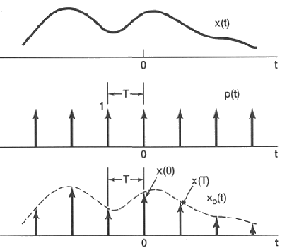
The sampling theorem

The sampling process of a continuous function x(t) can be represented by

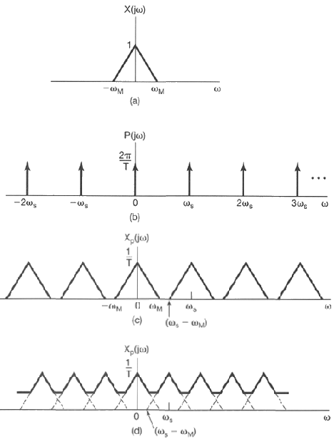
According to the convolution theorem, the spectrum of the resultant signal is

This convolution is very easy to carry out as P(f) is composed of a sequency of impulses. Note that after sampling x_s(t) becomes discrete and its spectrum becomes periodic accordingly.

Now the sampling theorem can be easily obtained by observing the result above. Note that only when the sampling rate f_s is more than twice the highest frequency component f_max of the signal (called Nyquist frequency, can the signal be recovered from its discrete samples (by ideal low-pass filtering). Otherwise, some high frequency components in the signal will be mixed with some low frequency components, i.e., aliasing occurs, and the signal can never be reconstructed without error.

To eliminate or reduce aliasing, we can

• Increase the sampling rate f_s=1/T_s by reducing T, or/and
• Reduce the high frequency component f_max contained in the signal by low-pass filtering it before sampling.