Next: Appendix A: Kullback-Leibler (KL)
Up: MCMC
Previous: Metropolis-Hastings sampling
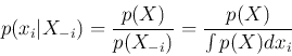
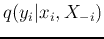
In M-H sampling,  can be updated one component at a time, so that
each iteration will take
can be updated one component at a time, so that
each iteration will take  steps each for one of the components
of . In this case, all distributions in the expression for the
acceptance probablity are for the i-th component
steps each for one of the components
of . In this case, all distributions in the expression for the
acceptance probablity are for the i-th component  of the random
vector conditioned on the remaining
of the random
vector conditioned on the remaining  components:
where
contains all the components except the i-th one. Moreover, the proposal
distribution in the i-th step of the t-th iteration becomes
where
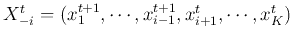 with its first
  components updated while the rest not. The
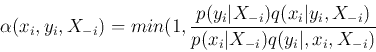
probability for acceptance is
components updated while the rest not. The
probability for acceptance is
In particular, if the proposal distribution
 is chosen
to be just the same as
is chosen
to be just the same as  , i.e.,
then the second term in the expression for the acceptance probability
becomes 1 and the sample generated by the proposal distribution is
always accepted. This particular version of the M-H method is the
Gibbs sampling, based on the assumption that the conditional
distribution
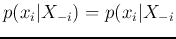 is simple enough to draw
samples from directly, although the whole distribution
is simple enough to draw
samples from directly, although the whole distribution  in
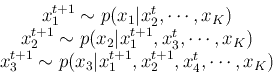
dimensional space is too complex to sample. The
iteration in Gibbs sampling in a dimensional space can be
illustrated as this:
in
dimensional space is too complex to sample. The
iteration in Gibbs sampling in a dimensional space can be
illustrated as this:
Gibbs sampling can be best illustrated in 2D space where the above
iteration becomes alternating sampling between the horizontal direction
for  and the vertical direction for
  . For example, if
is a 2D Gaussian, then the iteration will keep sampling the two 1D
Gaussians
. For example, if
is a 2D Gaussian, then the iteration will keep sampling the two 1D
Gaussians  and
and  alternatively along the sequence
of
alternatively along the sequence
of
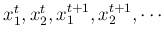 .
.
Next: Appendix A: Kullback-Leibler (KL)
Up: MCMC
Previous: Metropolis-Hastings sampling
Ruye Wang
2018-03-26