A 2D DFT Example

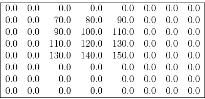
Consider a real 2D signal (imaginary part is zero):

$$\begin{tabular}{\vert rrrrrrrr\vert} \hline 0.0 & 0.0 & 0.0 ... ...0.0 & 0.0 & 0.0 & 0.0 & 0.0 & 0.0 & 0.0 \hline \end{tabular}$$

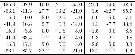
The real part of the spectrum:

$$\begin{tabular}{\vert r\vert rrr\vert r\vert rrr\vert} \hlin... ...2.7 & 1.6 & -21.0 & 13.2 & 27.7 & -11.3 \hline \end{tabular}$$

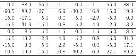
The imaginary part of the spectrum:

$$\begin{tabular}{\vert r\vert rrr\vert r\vert rrr\vert} \hlin... ....0 & -16.8 & 30.2 & -6.9 & 27.1 & -89.2 \hline \end{tabular}$$

Note that both the real and imaginary parts of the spectrum have some 2D symmetric property, indicating that half of the data is redundant. In time domain, the imaginary part is all zero, and in frequency domain, both real and imaginary parts are symmetric. This suggests that we can improve the 2D DFT algorithm by cutting the required computation by half.