Histogram Equalization

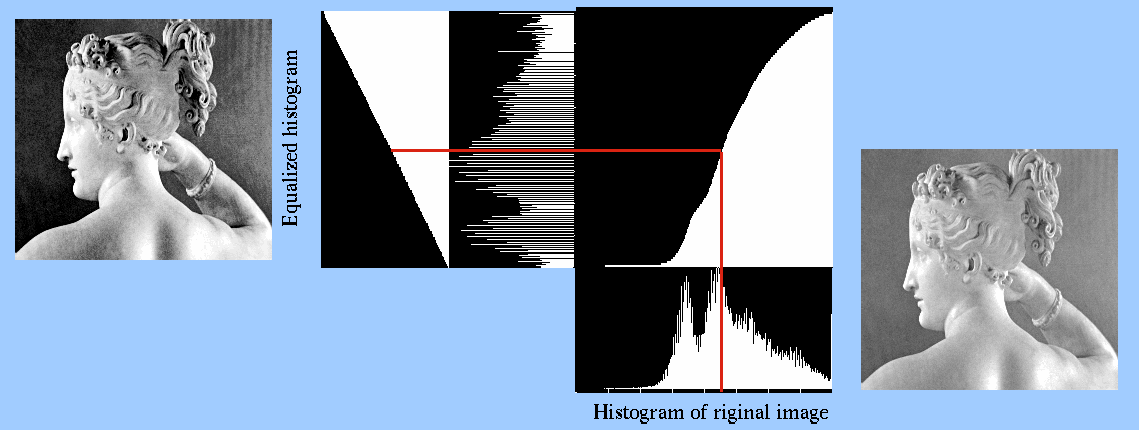
To transform the gray levels of the image so that the histogram of the resulting image is equalized to become a constant:

$$h[i]=\frac{1}{L}= ,\;\;\;\;\;\;0\le i\le L-1$$ (6)

The purposes:

• To make equal usage of all available gray levels in the dynamic range;
• To further modify the histogram.

We first assume the pixel values are continuous in the range of $0<x<1$, and a function $y=f(x)$ maps $x$ to $y$ also in the same range. We also assume all pixels within the gray scale interval $dx$ of the input image are mapped to the corresponding range $dy$ of the output image. As the number of pixels being mapped remains unchanged, we have

$$p(y)dy=p(x)dx$$ (7)

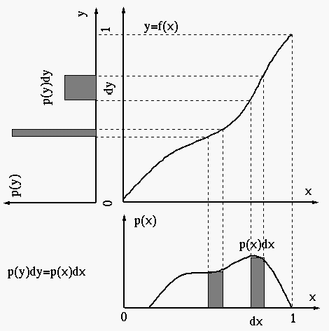
For the histogram of the output image to be equalized, it needs to be constant 1, i.e., $p(y)=1$, so that

$$\int_0^1 p(x)\;dx=\int_0^1 dy=1$$ (8)

We therefore have:

$$p(y)dy=dy=p(x)dx,\;\;\; \;\;\;\frac{dy}{dx}=p(x)$$ (9)

Integrating both sides, we get the mapping function $y=f(x)$ for the histogram equalization:

$$y=f(x)=\int_0^x p(u) du=P(x)-P(0)=P(x)$$ (10)

where $P(x)$ is the cumulative distribution of the gray levels of the input image:

$$P(x)=\int_0^x p(u) du, \;\;\;\;\;P(0)=0,\;\;\;\;\;\;P(1)=1$$ (11)

This histogram equalization mapping can be intuitively understood by checking the following two cases while both need to keep $p(y)dy=p(x)dx$:

• If $p(x)$ is low, $P(x)$ has a shallow slope, then $dy$ is narrow and $p(y)$ is high;
• If $p(x)$ is high, $P(x)$ has a steep slope, then $dy$ is wide and $p(y)$ is low.

i.e., the mapping maps high $p(x)$ to low $p(y)$ and low $p(x)$ to high $p(y)$, i.e., it tends to make $p(y)$ a flat curve, a uniform distribution.

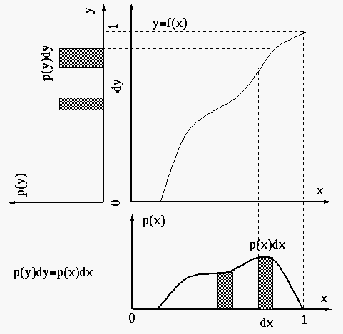
For discrete gray levels, the gray level of the input $x$ takes one of the $L$ discrete values: $0\le x < L$, and the continuous mapping function becomes discrete:

$$y'[j]=H_x[j]\stackrel{\triangle}{=}\sum_{i=0}^j h_x[i]$$ (12)

where $h_x[i]$ and $H_x[j]$ are respectively the density and cumulative histogram of the input image $x$:

$$h_x[i]=\frac{n_i}{\sum_{i=0}^{L-1} n_i} =\frac{n_i}{N},\;\;\;\;\;\;\; H_x[j]=\sum_{i=0}^j h_x[i],\;\;\;\;\;\;H_x[L-1] =\sum_{i=0}^{L-1} h_x[i]=1$$ (13)

and $n_i$ is the number of pixels with gray level $i$, and $N$ is the total number of pixels.

The resulting function $y'$ in the range $0 \le y' \le 1$ needs to be converted to the gray levels $0 \le y <L$ by either of the two ways:

1. $$y_1=\lfloor (L-1)\;y' +0.5 \rfloor$$ (14)

2. $$y_2=\lfloor (L-1) \;\frac{y'-y'_{min}}{1-y'_{min}}+0.5 \rfloor$$ (15)

where $\lfloor w \rfloor$ is the floor of a real number $w$ (the largest integer smaller than $w$), and adding $0.5$ is for proper rounding. Note that both conversions map $y'_{max}=1$ to the highest gray level $L-1$, but the second conversion also maps $y'_{min}$ to 0 to stretch the gray levels of the output image to occupy the entire dynamic range $0 \le y <L$; i.e., the second method does gray scale stretch as well as histogram equalization.

Example:

Assume the images have $N=64 \times 64=4096$ pixels in $L=8$ gray levels. The following table shows the equalization process corresponding to the two conversion methods above:

$$\begin{array}{c\vert c\vert\vert c\vert c\vert\vert c\vert c\... ...times 7=7 & 0.11 & 1.00 & 7 & 0.11 & 1.00 \\ \hline \end{array}$$ (16)

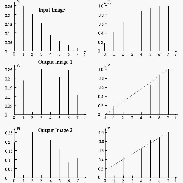
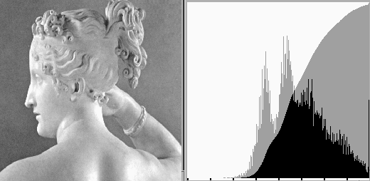
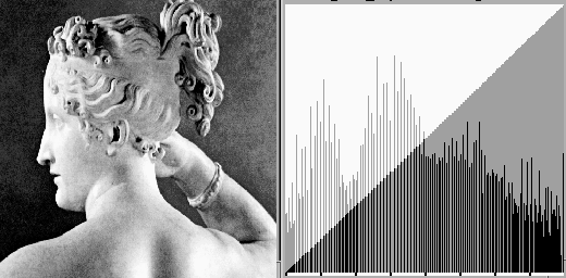
In the following example, the histogram of a given image is equalized. Although the resulting histogram may not look constant due to the discrete nature of the digital image, the cumulative histogram is an exact linear ramp indicating that the density histogram is indeed equalized. The density histogram is not guaranteed to be a constant because the pixels of the same gray level cannot be separated to satisfy a constant distribution.

Build lookup table:

      sum=0.0;
      for (i=0; i<256; i++) {
          sum=sum+h[i];
          lookup[i]=sum*255;
      }

Image Mapping:

    for (m=0; m<M; m++) 
        for (n=0; n<N; n++) 
            y[m][n]=lookup[x[m][n]];

Example: