Next: Transform Coding (lossy) and
Up: Inter-pixel Redundancy and Compression
Previous: Gray Level Image Compression
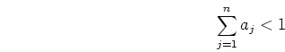
As natural signals are highly correlated, the difference between neighboring
samples is usually small. The value of a pixel x can be therefore predicted
by its neighbors a, b, c, and d with a small error:
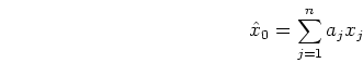
In general, the predicted value  for a pixel
  is a linear combination
of all available neighbors
is a linear combination
of all available neighbors
 :
:
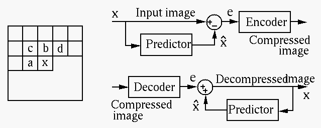
The entropy of the histogram of the error image hist(e) is much smaller than
that of the histogram of the original image hist(x), therefore Huffman coding
will be much more effective for the error image than the original one.
Optimal predictive coding
The mean square error of the predictive error is:
where
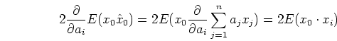
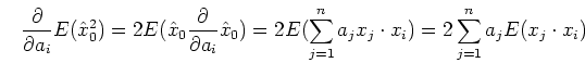
To find the optimal coefficients  so that
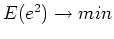 is minimized,
we let
is minimized,
we let
but as
and
we have
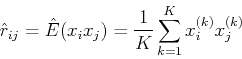
Here
is the correlation between  and
and  which can be estimated from data obtained
from multiple trials:
which can be estimated from data obtained
from multiple trials:
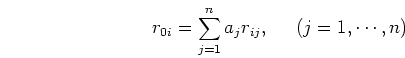
Now the optimal prediction above can be written as
which can be expressed in vector form:
where
Then the coefficients can be found as
To prevent predictive error from being accumulated, we require
so that the errors will not propagate.
Examples
where
Next: Transform Coding (lossy) and
Up: Inter-pixel Redundancy and Compression
Previous: Gray Level Image Compression
Ruye Wang
2021-03-28

![\begin{displaymath}{\bf r}_0=\left[ \begin{array}{c}r_{01} \cdots r_{0n} \...
... ... & r_{ij} & ... \\
... & ... & ... \end{array} \right]
\end{displaymath}](img155.png)