Next: Information conservation in feature
Up: Feature Selection
Previous: Optimal transformation for maximizing
The previous method only maximizes the between-class scatteredness  without taking into consideration the within-class scatteredness
  ,
or, equivalently, the total scatteredness
,
or, equivalently, the total scatteredness
 . As
it is possible that in the space after the transform
. As
it is possible that in the space after the transform
 the between-class scatteredness
 is maximized but so is the
total scatteredness
is maximized but so is the
total scatteredness
 , while it is desirable to maximize
and minimize at the same time in order to maximize
the separability. A better criterion for feature selection can be
, while it is desirable to maximize
and minimize at the same time in order to maximize
the separability. A better criterion for feature selection can be
![$J=tr[{\bf S}_W^{-1}{\bf S}_B]$](img399.png) as it relative separability.
as it relative separability.
In order to find the optimal transform matrix
![${\bf A}=[{\bf a}_1,\cdots,{\bf a}_M]$](img18.png) ,
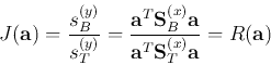
we consider the maximization of the objective function
,
we consider the maximization of the objective function  :
:
where
and
Note that as
 is not symmetric (the product of two symmetric
matrices is in general not symmetric), the KLT method used for the maximization
of
is not symmetric (the product of two symmetric
matrices is in general not symmetric), the KLT method used for the maximization
of
 considered previously can no longer be used to maximize
 .
.
To find the transform matrix  so that
![$J({\bf A})=tr\;[ ({\bf S}_T^{(y)})^{-1}{\bf S}_B^{(y)}]$](img408.png) is maximized, we first
consider the case of
is maximized, we first
consider the case of  to find a single feature
 ,
obtained by an
,
obtained by an  vector
 . The objective function
above becomes
. The objective function
above becomes
This function of  is the
Rayleigh quotient
is the
Rayleigh quotient
 of the two symmetric matrices
 and
and
 . The optimal
transform vector that maximizes
. The optimal
transform vector that maximizes  can be found by solving
the corresponding
generalized eigenvalue problem
can be found by solving
the corresponding
generalized eigenvalue problem
or in matrix form:
where
![${\bf\Phi}=[{\bf\phi}_1,\cdots,{\bf\phi}_N]$](img421.png) , and
, and  is the
ith eigenvector of
is the
ith eigenvector of
![${\bf S}_{B/T}=[{\bf S}_T^{(x)}]^{-1}{\bf S}_B^{(x)}$](img422.png) , and the
corresponding eigenvalue is
, and the
corresponding eigenvalue is
 , which is maximized
by the eigenvector
, which is maximized
by the eigenvector
 (
( ) corresponding to
the greatest eigenvalue
) corresponding to
the greatest eigenvalue  .
.
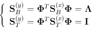
By solving the above generalized eigen-equation, we get the eigenvector matrix
 , which can be used as the linear transform matrix by
which both
and
can be diagonalized at the same
time:
, which can be used as the linear transform matrix by
which both
and
can be diagonalized at the same
time:
and we get
We can therefore construct a transform matrix
![${\bf\Phi}_{N\times M}=[{\bf\phi}_1,
\cdots,{\bf\phi}_M]$](img429.png) composed of the
composed of the  eigenvectors
  corresponding
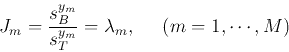
to the largest eigenvalues the Rayleigh quotient
corresponding
to the largest eigenvalues the Rayleigh quotient
 representing the separability in the mth
dimension for
representing the separability in the mth
dimension for
 , (
, ( ), so that in the resulting
M-D space,
), so that in the resulting
M-D space,
- the signal components in
 are completely
decorrelated, i.e., they each carry some separability information independent
of others.
are completely
decorrelated, i.e., they each carry some separability information independent
of others.
- the separability along each signal component
 is
maximized
is
maximized
The generalized eigen-equation above can be further written as
where  is a diagonal matrix composed of
 on its diagonal:
We see that using the greatest eigenvalues  of
of  to
maximize is equivalent to using the greatest eigenvalues
to
maximize is equivalent to using the greatest eigenvalues
 of
of  to maximize .
Next: Information conservation in feature
Up: Feature Selection
Previous: Optimal transformation for maximizing
Ruye Wang
2016-11-30