Optimal transformation for maximizing $tr({\bf S}_B)$

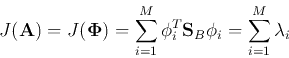
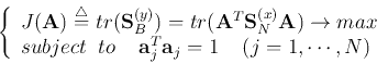
First we realize that the separability criterion $tr\;({\bf S}_B^{(y)})$ in the space ${\bf y}={\bf A}^T {\bf x}$ can be expressed as:

$$J^{(y)}({\bf A}) = tr\;({\bf S}_{B}^{(y)}) = tr\;({\bf A}^T {\bf S}_{B}^{(x)} {\bf... ...s {\bf a}_N^T\end{array} \right]{\bf S}_B^{(x)}[{\bf a}_1,\cdots,{\bf a}_N]$$

$$= tr \; \left[ \begin{array}{c} {\bf a}_1^T \vdots {\bf a}_N... ...{\bf S}_{B}^{(x)}{\bf a}_N] =\sum_{i=1}^N {\bf a}_i^T{\bf S}_B^{(x)}{\bf a}_i$$

The optimal transform matrix ${\bf A}$ which maximizes $tr({\bf S}_B^{(y)})$ can be obtained by solving the following optimization problem:

$$\left\{ \begin{array}{l} J({\bf A})\stackrel{\triangle}{=}... ..._j^{T}{\bf a}_j=1 \;\;\;\;(j=1, \cdots, N) \end{array} \right.$$

Here we have further assumed that ${\bf A}$ is an orthogonal matrix (a justifiable constraint as orthogonal matrices conserve energy/information in the signal vector). This constrained optimization problem can be solved by Lagrange multiplier method:

$$\frac{\partial}{\partial {\bf a}_i}\left[J({\bf A})-\sum_{j=1}^N ... ...}_j^T{\bf S}_B^{(x)}{\bf a}_j-\lambda_j {\bf a}_j^T{\bf a}_j+\lambda_j) \right]$$

$$= \frac{\partial}{\partial {\bf a}_i} \left[{\bf a}_i^T{\bf S}_B^{... ...\bf a}_i^T{\bf a}_i \right] = 2{\bf S}_B^{(x)}{\bf a}_i-2\lambda_i{\bf a}_i =0$$

We see that the column vectors of ${\bf A}$ must be the orthogonal eigenvectors of the symmetric matrix ${\bf S}_{B}$:

$${\bf S}_B{\bf a}_i=\lambda_i{\bf a}_i \;\;\;\;\;\;(i=1, \cdots, N)$$

i.e., the transform matrix must be

$${\bf A}=[{\bf a}_1, \cdots,{\bf a}_N]={\bf\Phi}=[{\bf\phi}_1, \cdots, {\bf\phi}_N]$$

Thus we have proved that the optimal feature selection transform is the principal component transform (KLT) which, as we have shown before, tends to compact most of the energy/information (representing separability here) into a small number of components. Therefore the $M$ new features can be obtained by

$${\bf y}_{M\times 1}={\bf A}_{M\times N}^T {\bf x}_{N\times ... ...\phi}^T_M \end{array} \right]_{M\times N} {\bf x}_{N\times 1}$$

and

$$J({\bf A})=J({\bf\Phi})=\sum_{i=1}^M {\bf\phi}_i^T{\bf S}_B{\bf\phi}_i = \sum_{i=1}^M \lambda_i$$

Obviously, to maximize $J({\bf A})$, we just need to choose the $M$ eigenvectors ${\bf\phi}_i$'s corresponding to the $m$ largest eigenvalues of ${\bf S}_{B}$:

$$\lambda_1 \geq \lambda_2 \geq \cdots \geq \lambda_M \geq \cdots \geq \lambda_N$$

In the subspace spanned by these $m<n$ new features, $tr({\bf S}_B)$ with be maximized.