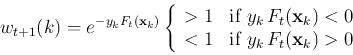
The Adaptive boosting (AdaBoost) is a supervised binary
classification algorithm based on a training set
![]() , where each sample
, where each sample
![]() is labeled by
is labeled by
![]() , indicating to which
of the two classes it belongs.
, indicating to which
of the two classes it belongs.
AdaBoost is an iterative algorithm. In the t-th iterative step, a
weak classifier, considered as a hypothesis and denoted by
![]() , is to be used to classify each of
the
, is to be used to classify each of
the ![]() training samples into one of the two classes. If a sample
training samples into one of the two classes. If a sample
![]() is correctly classified,
is correctly classified,
![]() ,
i.e.,
,
i.e.,
![]() ; if it is misclassified,
; if it is misclassified,
![]() , i.e.,
, i.e.,
![]() .
We need to find the best weak classifier that minimizes the
weighted error rate defined as:
.
We need to find the best weak classifier that minimizes the
weighted error rate defined as:
 |
|||
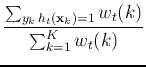 |
The classifier is weak in the sense that its performance only needs
to be better than chance, i.e., the error rate defined above is less
than 50 percent,
![]() .
.
At each iteration, a strong or boosted classifier ![]() can also be constructed based on the linear combination of all
previous weak classifiers
can also be constructed based on the linear combination of all
previous weak classifiers
![]() :
:

![\begin{displaymath}
H_t({\bf x})=sign [F_t({\bf x})]=\left\{\begin{array}{ll}
+1 & F_t({\bf x})>0 -1 & F_t({\bf x})<0\end{array}\right.
\end{displaymath}](img234.png)
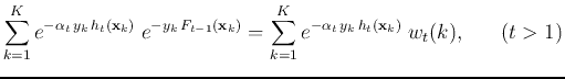
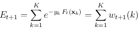
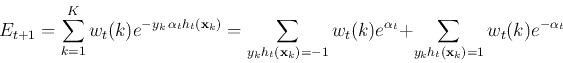
The performance of the strong classifier can be measured by the
exponential loss defined as
![$\displaystyle \sum_{k=1}^K e^{-y_k F_t({\bf x}_k)}
=\sum_{k=1}^K e^{-y_k [\alpha_t h_t({\bf x}_k)+F_{t-1}({\bf x}_k)]}$](img237.png) |
|||
 |
We see that ![]() of the t-th iteration can be obtained
recursively from
of the t-th iteration can be obtained
recursively from ![]() of the previous iteration, and
this recursion can be carried out all the way back to the first
step
of the previous iteration, and
this recursion can be carried out all the way back to the first
step ![]() with
with
![]() .
.
Following this recursive definition of the weights, the exponential
loss defined above can be written as the sum of all ![]() weights:
weights:
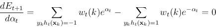
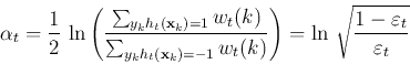
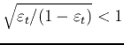
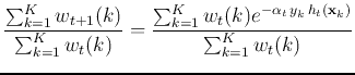
We need to further determine the optimal coefficient ![]() in the function
in the function ![]() that minimizes the exponential
loss
that minimizes the exponential
loss ![]() . To do so, we first separate the summation for
. To do so, we first separate the summation for ![]() into
two parts, for the samples that are classified by
into
two parts, for the samples that are classified by ![]() correctly
and incorrectly:
correctly
and incorrectly:
 and
and
As the strong classifier ![]() takes advantage of all previous weak
classifiers
takes advantage of all previous weak
classifiers
![]() , each of which may be more effective in
a certain region of the N-D space than others,
, each of which may be more effective in
a certain region of the N-D space than others, ![]() can be expected
to be a much more accurate classifier than any of the weak classifiers.
Also note that a
can be expected
to be a much more accurate classifier than any of the weak classifiers.
Also note that a ![]() with a smaller error
with a smaller error ![]() will be
weighted by a greater
will be
weighted by a greater ![]() and therefore contribute more to the
strong classifier
and therefore contribute more to the
strong classifier ![]() , but a
, but a ![]() with a large
with a large ![]() will
be weighted by a smaller
will
be weighted by a smaller ![]() and contributes less to
and contributes less to ![]() .
.
Having found the optimal coefficient
 , we can further
get
, we can further
get
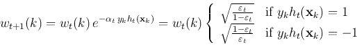
 if it is classified
correctly
if it is misclassified
if it is classified
correctly
if it is misclassified
We further consider the ratio of the exponential losses of
two consecutive iterations:
 |
|||
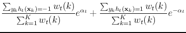 |
|||
 |
The weak classifier used in each iteration is typically implemented
as a decision stump, a binary classifier that partitions the
N-D feature space into two regions. Specifically, a coordinate descent
method is used by which all samples in the training set are projected
onto ![]() , one of the
, one of the ![]() dimensions of the feature space:
dimensions of the feature space:
![\begin{displaymath}
\varepsilon_t=\sum_{k=1}^K w_t(k)\; I[h_t(x_k)\ne y_k]
\end{displaymath}](img278.png)
Alternatively, the weak classifier can also obtained based on the
principal component analysis (PCA) by partitioning the N-D feature
space along the directions of the eigenvectors of the between-class
scatter matrix
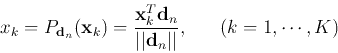
Example 1 Consider the classification of two classes of ![]() simples in 2-D space, shown as red and blue dots in the figure below,
which are not linearly separable. As shown in the figure, the 2-D
space is partitioned along both the standard basis vectors (left) and
the PCA directions (right). The PCA method performances significantly
better in this example as its error reduces faster and it converges
to zero after 61 iterations, while the error of the method based on
the standard axes (in vertical and horizontal directions) does not
go down to zero even after 120 iterations. This more faster reduction
of error of the PCA method can be easily understood as many different
directions are used to partition the space into two regions, while the coordinate
method
simples in 2-D space, shown as red and blue dots in the figure below,
which are not linearly separable. As shown in the figure, the 2-D
space is partitioned along both the standard basis vectors (left) and
the PCA directions (right). The PCA method performances significantly
better in this example as its error reduces faster and it converges
to zero after 61 iterations, while the error of the method based on
the standard axes (in vertical and horizontal directions) does not
go down to zero even after 120 iterations. This more faster reduction
of error of the PCA method can be easily understood as many different
directions are used to partition the space into two regions, while the coordinate
method
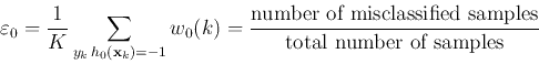
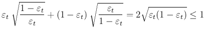
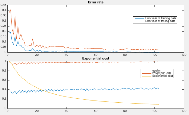
How the AdaBoost is iteratively trained can be seen in the figure below.
First, the error rate, the ratio between the number of misclassified
samples and the total number of samples, for both the training and
testing samples, are plotted as the iteration progresses (top). Also,
the weighted error ![]() , the exponential costs
, the exponential costs ![]() ,
and the ration
,
and the ration
 are
all ploted (bottom). We see that
are
all ploted (bottom). We see that
![]() and
and ![]() for all steps, and the exponential cost
for all steps, and the exponential cost ![]() attenuates exponentially
towards zero.
attenuates exponentially
towards zero.
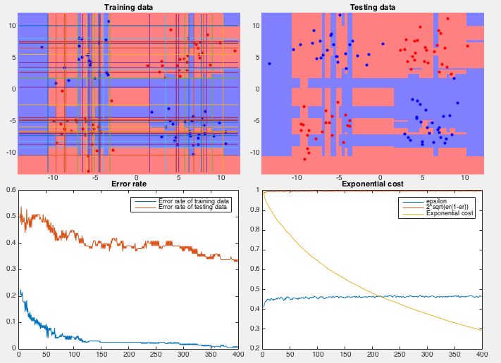
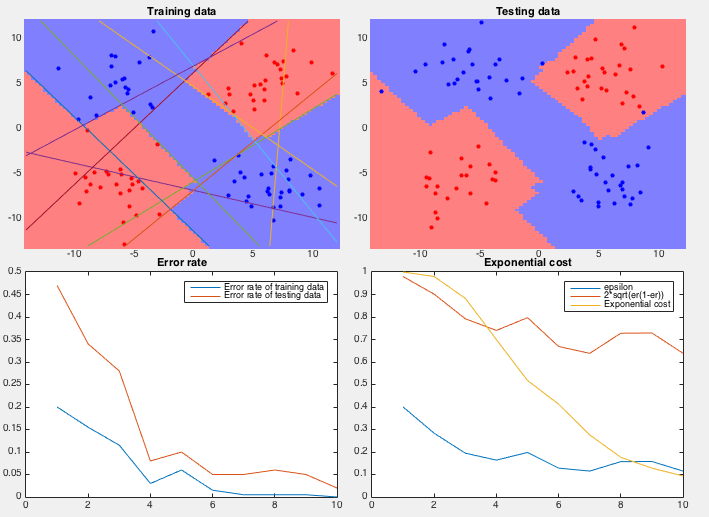
Example 2 In this dataset, 100 training samples of two classes (50 each) forms four clusters arranged in the 2-D space as an XOR pattern as shown figure (top-left), and 100 testing samples of the same distribution are classified by the AbaBoost algorithm trained by both the coordinate descent and PCA methods.
We see that the coordinate descent method performs very poorly in both the slow convergence (more than 400 iterations) during training and high classification error rate (more than 1/3) during testing. The partitioning of the 2-D space is an obvious over fitting of the training set instead of reflecting the actual distribution of the two classes (four clusters). On the other hand, the PCA method converges quickly (only 10 iterations) and classifies the testing samples with very low error rate. The space is clearly partitioned into two regions corresponding to the two classes.