


Next: Pseudo-inverse
Up: algebra
Previous: Normal matrices and diagonalizability
SVD Theorem: An  matrix
  of rank
  can be diagonalized by two unitary matrices
 and
and
 :
:
where
-
![${\bf U}_{M\times M}=[{\bf u}_1,\ldots,{\bf u}_M]$](img377.png) is a unitary
matrix (
is a unitary
matrix (
 ) composed of the left
singular vectors satisfying
) composed of the left
singular vectors satisfying
or in matrix form
-
![${\bf V}_{N\times N}=[{\bf v}_1,\ldots,{\bf v}_N]$](img381.png) is a unitary
matrix (
is a unitary
matrix (
 ) composed of the right
singular vectors satisfying
) composed of the right
singular vectors satisfying
or in matrix form
-
 is an diagonal matrix
with
is an diagonal matrix
with  non-zero singular values

 of
of
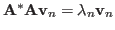
Proof: Let  and
and  be the nth eigenvalue and
the corresponding normalized eigenvector of the
be the nth eigenvalue and
the corresponding normalized eigenvector of the  matrix
 satisfying the following eigenequation:
As
 is Hermitian (symmetric if
is real), its eigenvalues are real and its
normalized eigenvectors are orthonormal:
is Hermitian (symmetric if
is real), its eigenvalues are real and its
normalized eigenvectors are orthonormal:
 ,
i.e., the eigenvector matrix defined as
is unitary
(orthogonal if is real):
,
i.e., the eigenvector matrix defined as
is unitary
(orthogonal if is real):
The eigenequation can be written in matrix form:
where
![${\bf\Lambda}=diag[\lambda_1,\cdots,\lambda_N]$](img398.png) .
.
Pre-multiplying on both sides of
 we get
We see that
 is the eigenvector of the Hermitian matrix
 corresponding to its eigenvalue , with norm:
We define the normalized eigenvector of
as
As
is Hermitian, its normalized eigenvectors are
orthonormal, which can also be shown as:
We define
which is also unitary
Now we have
Q.E.D.
When
 is Hermitian (symmetric if real), i.e.,
 , then if
we also have
i.e., the singular values
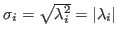 are
the absolute values of its eigenvalues
are
the absolute values of its eigenvalues
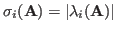 ,
and
,
and
 .
.
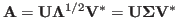
The SVD equation
can be considered as the forward SVD transform. Pre-multiplying  and
post-multiplying
and
post-multiplying  on both sides, we get the inverse transform:
by which the original matrix is represented as a linear combination
of matrices
![$[{\bf u}_k{\bf v}_k^*]$](img418.png) weighted by the singular values
weighted by the singular values
 (
( ). We can rewrite both the forward and
inverse SVD transform as a pair of forward and inverse transforms:
). We can rewrite both the forward and
inverse SVD transform as a pair of forward and inverse transforms:
Given the SVD of an matrix
 ,
its pseudo-inverse can be found to be
,
its pseudo-inverse can be found to be
where
 is pseudo-inverse of
  , composed of
the reciprocals
, composed of
the reciprocals  of the singular values along the diagonal.
The matrix
 can be
considered as alinear transformation that converts a vector
can be
considered as alinear transformation that converts a vector
 to another vector
 in three steps:
- Rotate vector
 by the unitary matrix :
- Scale each dimention
 of
of  by a factor of
  ():
():
- Rotate vector
 by the unitary matrix :

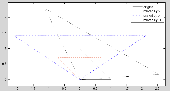
The figure below illustrates the transformation of the three vertices of
a triangle in 2-D space by a matrix
 ,
which first rotates the vertices by 45 degrees CCW, scale horitontally and
vertically by a factor of 3 and 2, respectively, and then rotate CW by 30
degrees.
,
which first rotates the vertices by 45 degrees CCW, scale horitontally and
vertically by a factor of 3 and 2, respectively, and then rotate CW by 30
degrees.
Next: Pseudo-inverse
Up: algebra
Previous: Normal matrices and diagonalizability
Ruye Wang
2015-04-27
![\begin{displaymath}
{\bf A}={\bf U}{\bf\Sigma}{\bf V}^*
=[{\bf u}_1,\cdots\cdo...
...nd{array}\right]
=\sum_{k=1}^R \sigma_k[{\bf u}_k{\bf v}_k^*]
\end{displaymath}](img417.png)