For a decision hyper-plane
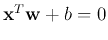 to separate the two
classes P
to separate the two
classes P  and N
and N
 , it has to satisfy
for both
 and
and
 . Among all such planes satisfying
this condition, we want to find the optimal one that separates the two
classes with the maximal margin (the distance between the decision plane
and the closest sample points).
. Among all such planes satisfying
this condition, we want to find the optimal one that separates the two
classes with the maximal margin (the distance between the decision plane
and the closest sample points).
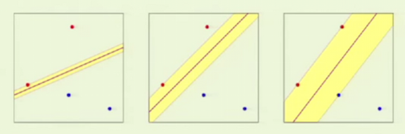
The optimal plane should be in the middle of the two classes, so that
the distance from the plane to the closet point on either side is the
same. We define two additional planes  and
and  that are parallel
to
that are parallel
to  and go through the point closet to the plane on either side:
All points
on the positive side should satisfy
and all points
on the negative side should satisfy
These can be combined into one inequality:
The equality holds for those points on the planes or . Such
points are called support vectors, for which
i.e., the following holds for all support vectors:
Moreover, the distances from the origin to the three planes ,
and are, respectively,
 ,
,
 , and
, and
 , and the distances between planes and is
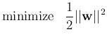
 , which is to be maximized. Now the problem of finding the
optimal decision plane in terms of
, which is to be maximized. Now the problem of finding the
optimal decision plane in terms of  and
and  can be formulated as:
Since the objective function is quadratic, this constrained optimization
problem is called a quadratic program (QP) problem.
(If the objective function is linear, the problem is a linear program (LP)
problem). This QP problem can be solved by Lagrange multipliers method to
minimize
with respect to , and the Lagrange coefficients
 . We let
These lead, respectively, to
Substituting these two equations back into the expression of
. We let
These lead, respectively, to
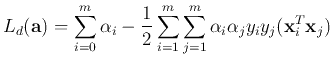
Substituting these two equations back into the expression of  ,
we get a simplified dual problem with respect to
,
we get a simplified dual problem with respect to  of the
above primal problem:
of the
above primal problem:
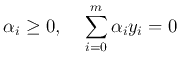
Here the objective function is only a function of the dot product
 . Once this quadratic programming problem is
solved for
. Once this quadratic programming problem is
solved for
 , we can find .
The dual problem is related to the primal problem by:
As  is the greatest lower bound (infimum) of
  for all
and , we want it to be maximized.
for all
and , we want it to be maximized.
Solving this dual problem (an easier problem than the primal one), we get
, from which of the optimal plane can be found.
Those points  on either of the two planes and
(for which the equality
on either of the two planes and
(for which the equality
 holds) are
called the support vectors and they correspond to positive
Lagrange multipliers
holds) are
called the support vectors and they correspond to positive
Lagrange multipliers  . The training depends only on the
support vectors, while all other samples away from the planes
and corresponding to
. The training depends only on the
support vectors, while all other samples away from the planes
and corresponding to  are farther away from the two
planes and they are not important.
are farther away from the two
planes and they are not important.
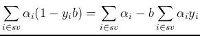
For a support vector (on the or plane), the
constraining condition is
where  is a set of all indices of support vectors .
Substituting
into the equation above we get
Note that the summation only contains terms corresponding to those
support vectors
is a set of all indices of support vectors .
Substituting
into the equation above we get
Note that the summation only contains terms corresponding to those
support vectors  with
with  . The parameter
can be found by solving the equation above based on any support
vector with .
. The parameter
can be found by solving the equation above based on any support
vector with .
For the optimal weight vector and optimal , we have:
The last equality is due to
 shown above.
Recall that the distance between the two margin planes and
is , and the margin, the distance between
(or ) and the optimal decision plane , is
shown above.
Recall that the distance between the two margin planes and
is , and the margin, the distance between
(or ) and the optimal decision plane , is