Kernel Mapping

The algorithm above converges only for linearly separable data. If the data set is not linearly separable, we can map the the samples ${\bf x}$ into a feature space of higher or even infinite dimensional space:

$${\bf x} \longrightarrow {\bf z}=\Phi({\bf x})$$

in which the classes can be linearly separated. The decision function in the new space becomes:

$$f({\bf x})=\Phi({\bf x})^T {\bf w}+b= \sum_{j=1}^m \alpha_j y_j (\phi({\bf x}_i)^T \phi({\bf x}_j))+b$$

where

$${\bf w}=\sum_{j=1}^m \alpha_j y_j \Phi({\bf x}_j)$$

and $b$ are the parameters of the decision plane in the new space. As the vectors ${\bf x}_i$ appear only in inner products in both the decision function and the learning law, the mapping function $\Phi({\bf x})$ does not need to be explicitly specified. Instead, all we need is the inner product of the vectors in the new space. The function $\Phi({\bf x})$ is a kernel-induced implicit mapping.

Definition: A kernel is a function that takes two vectors ${\bf x}_i$ and ${\bf x}_j$ as arguments and returns the value of the inner product of their images $\Phi({\bf x}_i)$ and $\Phi({\bf x}_j)$:

$$K({\bf x}_1,{\bf x}_2)=\phi({\bf x}_1)^T\phi({\bf x}_2)$$

As only the inner product of the two vectors in the new space is needed, we never need to actually carry out the computation of the inner product, i.e., the dimensionality of the new space (even infinite dimensional) is not important.

The learning algorithm in the kernel space can be obtained by replacing all inner products in the learning algorithm in the original space with the kernels:

$$f({\bf x})=\Phi({\bf x})^T {\bf w}+b=\sum_{j=1}^m \alpha_j y_j K({\bf x}_i,{\bf x}_j)+b$$

Example 1: linear kernel

Assume ${\bf x}=(x_1,\cdots,x_n)^T$, ${\bf z}=(z_1,\cdots,z_n)^T$,

$$K({\bf x},{\bf z})=({\bf x}^T {\bf z}+c)^n=\left(\sum_{i=1}^n x_iz_i+c\right)^n$$

Example 2: polynomial kernels

Assume ${\bf x}=(x_1,x_2)^T$, ${\bf z}=(z_1,z_2)^T$,

$$K({\bf x},{\bf z})=({\bf x}^T{\bf z})^2 = (x_1z_1+x_2z_2)^2=x_1^2z_1^2+x_2^2z_2^2+2x_1z_1x_2z_2$$

$$= [x_1^2,x_2^2,\sqrt{2}x_1x_2)]^T[z_1^2,z_2^2,\sqrt{2}z_1z_2] =\phi({\bf x})^T \phi({\bf z})$$

This is a mapping from a 2-D space to a 3-D space.

Example 3:

$$K({\bf x},{\bf z})=e^{-\vert\vert{\bf x}-{\bf z}\vert\vert^2/2\sigma^2}$$

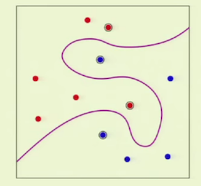
If the two classes are not linearly separable in the original n-D space of ${\bf x}$, they are more likely to be linearly separable in the higher dimensional space of ${\bf z}$. When mapped back to the original space, the two classes can be completely separated.

Caltech SVM

Caltech machine learning course