Linear separation of a feature space

This is a variation of the perceptron learning algorithm. Consider a hyper plane in an n-dimensional (n-D) feature space:

$$f({\bf x})={\bf x}^T {\bf w}+b=\sum_{i=0}^n x_i w_i+b=0$$

where the weight vector ${\bf w}$ is normal to the plane, and $b/\vert{\bf w}\vert$ is the distance from the origin to the plane. The n-D space is partitioned by the plane into two regions. We further define a mapping function $y=sign(f({\bf x})) \in \{1,-1\}$, i.e.,

$$f({\bf x})={\bf x}^T {\bf w}+b=\left\{ \begin{array}{ll} >0, & y... ...}\in P \\ <0, & y=sign(f({\bf x}))=-1,\;{\bf x}\in N \\ \end{array} \right.$$

Any point ${\bf x}\in P$ on the positive side of the plane is mapped to 1, while any point ${\bf x}\in N$ on the negative side is mapped to -1. A point ${\bf x}$ of unknown class will be classified to P if $f({\bf x})>0$, or N if $f({\bf x})<0$.

Given a set $m$ training samples from two linearly separable classes P and N:

$$\{ ({\bf x}_i, y_i), i=1,\cdots,m \}$$

where $y_i \in \{1,-1\}$ labels ${\bf x}_i$ to belong to either of the two classes. we want to find a hyper-plane in terms of ${\bf w}$ and $b$, by which the two classes can be linearly separated.

Before ${\bf w}$ is properly trained, the actual output $y'=sign(f({\bf x}))$ may not be the same as the desired output $y$. There are four possible cases:

$$\begin{tabular}{c\vert l\vert l\vert l} \hline & Input $({\bf x},... ...\hline 4 & $({\bf x},y=-1)$\ & $y'=-1= y $\ & corrrect \\ \hline \end{tabular}$$

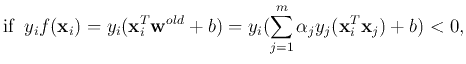
The two correct cases can also be summarized as

$$y f({\bf x})= y\, ({\bf x}^T {\bf w}+b)\ge 0$$

which is the condition a successful classifier should satisfy.

The weight vector ${\bf w}$ is updated whenever the result is incorrect (mistake driven):

• In case 2 above, $({\bf x},\;y=-1)$ but $y'=1\ne y$, then
  $${\bf w}^{new}={\bf w}^{old}+\eta y {\bf x}={\bf w}^{old}-\eta {\bf x}$$
  When the same ${\bf x}$ is presented again, we have
  $$f({\bf x})={\bf x}^T{\bf w}^{new}+b ={\bf x}^T{\bf w}^{old}-\eta {\bf x}^T{\bf x}+b<{\bf x}^T{\bf w}^{old}+b$$
  The output $y'=sign(f({\bf x}))$ is more likely to be $y=-1$ as desired. Here $0<\eta<1$ is the learning rate.
• In case 3 above, $({\bf x},\;y=1)$ but $y'=-1\ne y$, then
  $${\bf w}^{new}={\bf w}^{old}+\eta y {\bf x}={\bf w}^{old}+\eta {\bf x}$$
  When the same ${\bf x}$ is presented again, we have
  $$f({\bf x})={\bf x}^T{\bf w}^{new}+b ={\bf x}^T{\bf w}^{old}+\eta {\bf x}^T{\bf x}+b>{\bf x}^T{\bf w}^{old}+b$$
  The output $y'=sign(f({\bf x}))$ is more likely to be $y=1$ as desired.

Summarizing the two cases, we get the learning law:

$$\mbox{if} \;\;y\, f({\bf x})= y ({\bf x}^T{\bf w}^{old}+b)<0,\;\;\mbox{then}\;\; {\bf w}^{new}={\bf w}^{old}+\eta y {\bf x}$$

We assume initially ${\bf w}=0$, and the $m$ training samples are presented repeatedly, the learning law during training will yield eventually:

$${\bf w}=\sum_{j=1}^m \alpha_j y_j {\bf x}_j$$

where $\alpha_i>0$. Note that ${\bf w}$ is expressed as a linear combination of the training samples. After receiving a new sample $({\bf x}_i,y_i)$, vector ${\bf w}$ is updated by

$$\mbox{if} \;\;y_i f({\bf x}_i)=y_i ({\bf x}_i^T{\bf w}^{old}+b)=y_i(\sum_{j=1}^m \alpha_j y_j({\bf x}_i^T{\bf x}_j)+b)<0,$$

$$\mbox{then}\;\; {\bf w}^{new} ={\bf w}^{old}+\eta y_i {\bf x}_i=\... ...j +\eta y_i {\bf x}_i,\;\;\;\mbox{i.e.}\;\;\;\alpha_i^{new}=\alpha_i^{old}+\eta$$

Now both the decision function

$$f({\bf x})={\bf x}^T {\bf w}+b=\sum_{j=1}^m \alpha_j y_j ({\bf x}_i^T {\bf x}_j)+b$$

and the learning law

$$\mbox{if} \;\;y_i(\sum_{j=1}^m \alpha_j y_j({\bf x}_i^T{\bf x}_j)+b)<0,\;\;\; \mbox{then}\;\; \alpha_i^{new}=\alpha_i^{old}+\eta$$

are expressed in terms of the inner production of input vectors.