AdaBoost

The Adaptive boosting (AdaBoost) is a supervised binary classification algorithm based on a training set $\{ ({\bf x}_i,\,y_i)\;\vert\;i=1,\cdots,N\}$, where each sample ${\bf x}_i$ is labeled by $y_i\in\{-1,\,+1\}$, indicating to which of the two classes $C_-$ and $C_+$ it belongs.

AdaBoost is an iterative algorithm. In the t-th iteration, each of the $N$ training samples is classified into one of the two classes by a weak classifier $h_t({\bf x}_n)\in\{-1,\,+1\}$, which can be considered as a hypothesis. The classifier is weak in the sense that its performance only needs to be better than chance, i.e., the error rate is less than $50\%$. If a sample ${\bf x}_n$ is correctly classified, $h_t({\bf x}_n)=y_n=\pm 1$, i.e., $y_n\,h_t({\bf x}_n)=1$; if it is misclassified, $h_t({\bf x}_n)=-y_n=\pm 1$, i.e., $y_n\,h_t({\bf x}_n)=-1$. We need to find the best weak classifier that minimizes the weighted error rate defined as:

$$\varepsilon_t=\frac{\sum_{y_n\,h_t({\bf x}_n)=-1} w_t(n)}{\sum_{n=1}^N w_t(n)}$$ (41)

where $w_t(n)$ is the weight of the nth training samples at the t-th iteration. We can also get the correct rate:

$$1-\varepsilon_t=1-\frac{\sum_{y_n\,h_t({\bf x}_n)=-1} w_t(n)}{\sum_{n=1}^N w_t(n)} =\frac{\sum_{y_n\,h_t({\bf x}_n)=1} w_t(n)}{\sum_{n=1}^N w_t(n)}$$ (42)

At the initial stage with $t=0$, all $N$ samples are equally weighted by $w_0(1)=\cdots=w_0(N)=1$, and the weighted error

$$\varepsilon_0=\frac{1}{N} \sum_{y_n\,h_0({\bf x}_n)=-1} w_0(n) =\frac{\mbox{number of misclassified samples}} {\mbox{total number of samples}}$$ (43)

is actually the probability for any sample ${\bf x}$ in the training set to be misclassified by $h_0$. For the weak classifier the error rate defined above only needs to be lower than 50 percent, i.e., $\varepsilon_t<1/2$. When $t>0$, this weight $w_t(n)$ will be modified based on whether ${\bf x}_n$ is classified correctly in the subsequent iterations, as we will see below.

At each iteration, a strong or boosted classifier $H_t({\bf x}_n)$ is also constructed based on the linear combination (boosting) of all previous weak classifiers $h_1({\bf x}_n),\cdots, h_t({\bf x}_n)$ for all $n=1,\cdots,N$:

$$F_t({\bf x}_n) = \alpha_th_t({\bf x}_n)+F_{t-1}({\bf x}_n) =\alpha_th_t({\bf x}_n)+\alpha_{t-1}h_{t-1}({\bf x}_n)+F_{t-2}({\bf x}_n)$$

$$= \cdots=\sum_{i=1}^t\alpha_ih_i({\bf x}_n)$$ (44)

where the coefficient $\alpha_i$ for the weak classifier $h_i({\bf x}_n)$ in the i-th iteration is obtained as discussed below. Taking the sign function of $F_t({\bf x})$ we get the strong classifier:

$$H_t({\bf x}_n)=sign [F_t({\bf x}_n)]=\left\{\begin{array}{ll} +1 & F_t({\bf x}_n)>0\\ -1 & F_t({\bf x}_n)<0\end{array}\right.$$ (45)

which classifies a training sample ${\bf x}_n$ into one of the two classes, while the magnitude $\vert F_t({\bf x}_n)\vert$ represents the confidence of the decision.

The weight $w_t(n)$ of ${\bf x}_n$ in the t-th iteration $(t>0)$ is defined as

$$w_t(n)=e^{-y_n F_{t-1}({\bf x}_n)}\left\{\begin{array}{ll} >1 & \... ...ox{if $y_n\,F_{t-1}({\bf x}_n)>0$\ (correct classification)} \end{array}\right.$$ (46)

The weight $w_t(n)$ of the t-th iteration can be obtained recursively from $w_{t-1}(n)$ of the previous iteration:

$$w_t(n) = e^{-y_n\,F_{t-1}({\bf x}_n)} =e^{-y_n\,[\alpha_{t-1}h_{t-1}({\bf x}_n)+F_{t-2}({\bf x}_n)]}$$

$$= e^{-\alpha_{t-1}\,y_nh_{t-1}({\bf x}_n)}\;e^{-y_n\,F_{t-2}({\bf x}_n)} =e^{-\alpha_{t-1}\,y_nh_{t-1}({\bf x}_n)}\;w_{t-1}(n)$$ (47)

and this recursion can be carried out all the way back to the first iteration with $w_1(k)=e^{-\alpha_0 \,y_nh_0({\bf x}_n)}w_0(n)$.

The performance of the strong classifier can be measured by the exponential loss, defined as the sume of all $N$ weights:

$$E_{t+1}=\sum_{n=1}^N w_{t+1}(n)=\sum_{n=1}^N e^{-y_n\,F_t({\bf x}_n)} =\sum_{n=1}^N e^{-\alpha_t\,y_n\, h_t({\bf x}_n)} \;w_t(n) \;\;\;\;\;\;(t>1)$$ (48)

The coefficient $\alpha_t$ in Eq. (44) can now be found as the one that minimizes the exponential loss $E_{t+1}$. To do so, we first separate the terms in the summation for $E_{t+1}$ into two parts, corresponding to the samples that are classified by $h_t$ correctly and incorrectly:

$$E_{t+1}=\sum_{n=1}^N w_t(n)e^{-\alpha_t \,y_n\,h_t({\bf x}_n)} =\... ...f x}_n)=-1} w_t(n)e^{\alpha_t} +\sum_{y_n h_t({\bf x}_n)=1} w_t(n)e^{-\alpha_t}$$ (49)

and then set its derivative with respect to $\alpha_t$ to zero:

$$\frac{dE_{t+1}}{d\alpha_t} =\sum_{y_n h_t({\bf x}_n)=-1} w_t(n) e^{\alpha_t} -\sum_{y_n h_t({\bf x}_n)=1} w_t(n) e^{-\alpha_t}=0$$ (50)

Solving this equation we get $\alpha_t$ as the optimal coefficient that minimizes $E_{t+1}$:

$$\alpha_t=\frac{1}{2}\,\ln \left( \frac{\sum_{y_n h_t({\bf x}_n)=1... ...x}_n)=-1} w_t(n)}\right) =\ln\,\sqrt{\frac{1-\varepsilon_t}{\varepsilon_t}} > 0$$ (51)

which is greater than zero becauses $\varepsilon_t<1/2$, $1-\varepsilon_t>1/2$, and

$$e^{\alpha_t}=\sqrt{\frac{1-\varepsilon_t}{\varepsilon_t}}>1,\;\;\;\; e^{-\alpha_t}=\sqrt{\frac{\varepsilon_t}{1-\varepsilon_t}}<1$$ (52)

We now see that if a weak classifier $h_t$ has a small error $\varepsilon_t$, it will be weighted by a large $\alpha_t$ and therefore contributes more to the strong classifier $H_t$; on the other hand, if $h_t$ has a large error $\varepsilon_t$, it will be weighted by a small $\alpha_t$ and contributes less to $H_t$. As the strong classifier $H_t$ takes advantage of all previous weak classifiers $h_1,\cdots,h_t$, each of which may be more effective in a certain region of the N-D feature space than others, $H_t$ can be expected to be a much more accurate classifier than any of the weak classifiers.

Replacing $t$ by $t+1$ in Eq. (47), we now get

$$w_{t+1}(n)=w_t(n)\,e^{-\alpha_t\,y_nh_t({\bf x}_n)} =\left\{\begi... ..._t}{\varepsilon_t}}>w_t(n) & \mbox{if }y_n h_t({\bf x}_n)=-1 \end{array}\right.$$ (53)

We see that if $y_nh_t({\bf x}_n)=1$, i.e., ${\bf x}_n$ is classified correctly by $h_t$, it will be weighted more lightly by $w_{t+1}(n)<w_t(n)$ in the next iteration, but if $y_nh_t({\bf x}_n)=-1$, i.e., ${\bf x}_n$ is classified incorrectly by $h_t$, it will be weighted more heavily by $w_{t+1}(k)>w_t(k)$ in the next iteration, thereby it will be emphasized and have a better chance to be corrected to have more accurately classified by $h_{t+1}$ in the next iteration.

We further consider the ratio of the exponential losses of two consecutive iterations:

$$\frac{E_{t+1}}{E_t} = \frac{\sum_{n=1}^N w_{t+1}(n)}{\sum_{n=1}^N w_t(n)} =\frac{\sum_{n=1}^N w_t(n)e^{-\alpha_t\,y_n\,h_t({\bf x}_n)}}{\sum_{n=1}^N w_t(k)}$$

$$= \frac{\sum_{y_n h_t({\bf x}_n)=-1} w_t(n)}{\sum_{n=1}^N w_t(n)}e^... ...t} +\frac{\sum_{y_n h_t({\bf x}_n)=1} w_t(n)}{\sum_{n=1}^N w_t(n)}e^{-\alpha_t}$$

$$= \varepsilon_t\;\sqrt{\frac{1-\varepsilon_t}{\varepsilon_t}} +(1-\... ...c{\varepsilon_t}{1-\varepsilon_t}} =2\sqrt{\varepsilon_t(1-\varepsilon_t)}\le 1$$ (54)

This ratio is twice the geometric average $\sqrt{\varepsilon_t(1-\varepsilon_t)}\le 1$ of $\varepsilon_t$ and $1-\varepsilon_t$, which reaches its maximum when $\varepsilon_t=1-\varepsilon_t=1/2$. However, as $\varepsilon_t<1/2$, the ratio is always smaller than 1. We see that the exponential cost can be approximated as an exponentially decaying function from its initial value $E_0=\sum_{n=1}^N w_0(n)=N$ for some $\varepsilon<1/2$:

$$\lim_{t\rightarrow\infty}E_t\approx \lim_{t\rightarrow\infty}\left(2\sqrt{\varepsilon(1-\varepsilon)}\right)^t E_0=0$$ (55)

We can therefore conclude that the exponential loss will always decrease, i.e., the error of AdaBoost will always converge to zero.

The weak classifier used in each iteration is typically implemented as a decision stump, a binary classifier that partitions the N-D feature space into two regions. Specifically, as a simple example, a coordinate descent method can be used by which all training samples are projected onto the ith dimension of the feature space ${\bf d}_i$:

$$x_n=P_{{\bf d}_i}({\bf x}_n)=\frac{{\bf x}_n^T{\bf d}_i}{\vert\vert{\bf d}_i\vert\vert}, \;\;\;\;\;\;(n=1,\cdots,N)$$ (56)

and then classified into two classes by a threshold $T$ along the direction of ${\bf d}_i$:

$$h(x_n)=\left\{\begin{array}{ll}+1& \mbox{if }x_n<T\\ -1 & \mbox{if }x_n>T \end{array}\right.$$ (57)

The optimal decision stump is obtained when the following weighted error is minimized with respect to the threshold $T$ along that direction of ${\bf d}_i$:

$$\varepsilon_t=\sum_{n=1}^N w_t(n)\; \delta(h_t(x_n)-y_n) =\sum_{h_t(x_n)\ne y_n} w_t(n)$$ (58)

Alternatively, the weak classifier can also be obtained based on the principal component analysis (PCA) by partitioning the N-D feature space along the directions of the eigenvectors of the between-class scatter matrix

$${\bf S}_b=\frac{1}{N}\left[N_-({\bf m}_{-1}-{\bf m})({\bf m}_{-1}-{\bf m})^T +N_+({\bf m}_{+1}-{\bf m})({\bf m}_{+1}-{\bf m})^T\right]$$ (59)

where $N_-$ and $N_+$ are the numbers of samples in the two classes $(N_-+N_+=N)$, and

$${\bf m}_{\pm}=\frac{1}{N_{\pm}}\sum_{y_n=\pm 1} w(n)\,{\bf x}_n, \;\;\;\;\; {\bf m}=\frac{1}{N}\sum_{n=1}^N w(n)\,{\bf x}_n$$ (60)

are the weighted mean vectors of the two classes and the total weighted mean vector of all $N$ samples in the training set. The training samples are likely to be better separated along these directions of the eigenvectors of ${\bf S}_b$, which measures the separability of the two classes. The eigenequations of ${\bf S}_b$ is:

$${\bf S}_b={\bf\Phi\Lambda\Phi}^{-1}={\bf\Phi\Lambda\Phi}^T$$ (61)

As ${\bf S}_b$ is symmetric, the eigenvector matrix ${\bf\Phi}$ is orthonormal and its columns can be used as an orthogonal basis that spans the feature space as well as the standard basis. The same binary threshold classification considered above for the weak classifiers can be readily applied along these PCA bases.

The Matlab code of the main iteration loop of the algorithm is listed below, followed by the essential functions called by the main loop. Here T is the maximum number of iteration, and N is the total number of training samples.

The algorithm can be carried out in the feature space based on either the PCA basis (columns of the eigenvector matrix ${\bf\Phi}$), or the original standard basis (columns of the identity matrix ${\bf I}$).

The decision stump is implemented by a binary classifier, which partitions all training samples projected onto a 1-D space into two groups by a threshold value, which needs to be optimal in terms of the number of misclassification. A parameter plt is used to indicate the polarity of the binary classification, i.e., which of the two class $C_1$ and $C_0$ is on the lower (or higher) side of the threshold.

    Plt=[];              % polarity of binary classification
    Tr=[];               % transformation of basis vectors
    Th=[];               % threshold of binary classification
    Alpha=[];            % alpha values 
    h=zeros(T,N);        % h functions 
    F=zeros(T,N);        % F functions
    w=ones(T,N);         % weights for N training samples
    Er=N;                % error initialized to N
    t=0;                 % iteration index
    while t<T  & Er>0                 % the main iteration
        t=t+1;                        
        [tr th plt er]=WeakClassifier(X,y,w(t,:),PCA); % weak classifier
        alpha=log(sqrt((1-er)/er));   % update alpha   
        Alpha=cat(1,Alpha,alpha);     % record alpha
        Tr=cat(2,Tr,tr');             % record transform vector
        Th=cat(1,Th,th);              % record threshold 
        Plt=cat(1,Plt,plt);           % record polarity
        x=tr*X;                       % carry out transform
        c=sqrt(er/(1-er));
        for n=1:N                     % update weights
            h(t,n)=h_function(x(n),th,plt);     % find h function
           if  h(t,n)*y(n)<0
               w(t+1,n)=w(t,n)/c;     % update weights
           else
               w(t+1,n)=w(t,n)*c;
           end            
        end      
        F(t,:)=Alpha(t)*h(t,:);       % get F functions
        if t>1
            F(t,:)=F(t,:)+F(t-1,:);
        end
        Er=sum(sign(F(t,:).*y)==-1);  % error of strong classifier, number of misclassifications
        fprintf('%d: %d/%d=%f\n',t,Er,N,Er/N)
    end

Here are the functions called by the main iteration loop above:

function [Tr,Th Plt Er]=WeakClassifier(X,y,w,pca)
    % X: N columns each for one of the N training samples
    % y: labeling of X
    % w: weights for N training samples
    % pca: use PCA dimension if pca~=0
    % Er: minimum error among all D dimensions
    % Tr: transform vector (standard or PCA basis)
    % Th: threshold value 
    % Plt: polarity 
    [D N]=size(X);
    n0=sum(y>0);            % number of samples in class C+
    n1=sum(y<0);            % number of samples in class C-
    if pca                  % find PCA basis
        for i=1:D
            Y(i,:)=w.*X(i,:);
        end
        X0=Y(:,find(y>0));  % all samples in class C+
        X1=Y(:,find(y<0));  % all samples in class C-
        m0=mean(X0')';      % mean of C+
        m1=mean(X1')';      % mean of C-
        mu=(n0*m0+n1*m1)/N; % over all mean
        Sb=(n0*(m0-mu)*(m0-mu)'+n1*(m1-mu)*(m1-mu)')/N; % between-class scatter matrix
        [v d]=eig(Sb);      % eigenvector and eigenvalue matrices of Sb
    else
        v=eye(N);           % standard basis
    end  
    Er=9e9;
    for i=1:D               % for all D dimensions
        tr=v(:,i)';         % get transform vector from identity or PCA matrix
        x=tr*X;             % rotate the vector
        [th plt er]=BinaryClassifier(x,y,w); % binary classify N samples in 1-D
        er=0;
        for n=1:N
            h(n)=h_function(x(n),th,plt);  % h-function of nth sample 
            if h(n)*y(n)<0                 % if misclassified
                er=er+w(n);                % add error
            end
        end   
        er=er/sum(w);                      % total error of dimension d
        if Er>er                           % record info corresponding to min error
            Er=er;                         % min error
            Plt=plt;                       % polarity
            Th=th;                         % threshold
            Tr=tr;                         % transform vector
        end
    end 
end

function h=h_function(x, th, plt)
    if xor(x>th, plt)
        h=1;
    else
        h=-1;
    end
end

function [Th Plt Er]=BinaryClassifier(x,y,w)
    N=length(x); 
    [x1 i]=sort(x);            % sort 1-D data x
    y1=y(i);                   % reorder the targets 
    w1=w(i);                   % reorder the weights 
    Er=9e9;
    for n=1:N-1                % for N-1 ways of binary classification       
        e0=sum(w1(find(y1(1:n)==1)))+sum(w1(n+find(y1(n+1:N)==-1)));
        e1=sum(w1(find(y1(1:n)~=1)))+sum(w1(n+find(y1(n+1:N)~=-1)));
        if e1 > e0                 % polarity: left -1, right +1
            plt=0; er=e0; 
        else                       % polarity: left +1, right -1
            plt=1; er=e1;
        end
        if Er > er                 % update minimum error for kth dimension
            Er=er;                 % minimum error
            Plt=plt;               % polarity
            Th=(x1(k)+x1(k+1))/2;  % threshold
        end        
    end
end

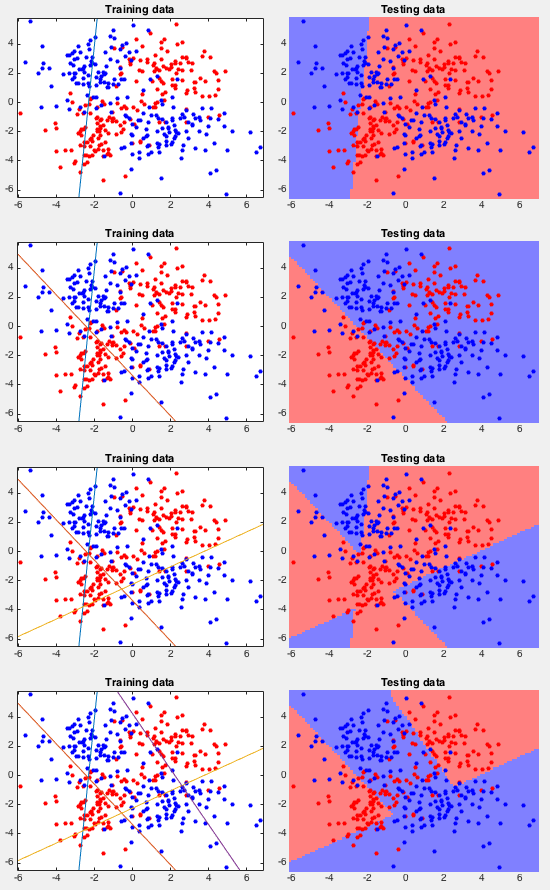
Example 0 This example shows the classification of an XOR data set (used previously the test the naive Bayes mehtod), containing two classes of $N=200$ simples each in 2-D space, represented by the red and blue dots in the figure below. The intermediate results after 4, 8, 16 and 32 iterations are shown in to illustrate the progress of the iteration, when the error rate continuously reduces from 134/400, 85/400, 81/400, 58/100.

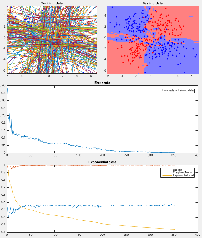
After over 350 iterations the error rate eventually reduced to zero (guaranteed by the AdaBoost method). The sequence of binary participation Although all training samples are correctly classified eventually, the result suffers the problem of overfitting.

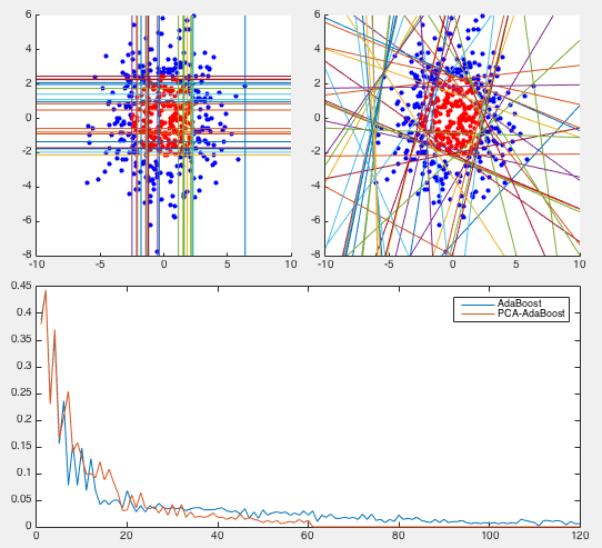
Example 1 This example shows the classification of two classes of $N=500$ simples in 2-D space, which is partitioned along both the standard basis vectors (left) and the PCA directions (right). The PCA method performances significantly better in this example as its error reduces faster and it converges to zero after 61 iterations, while the error of the method based on the standard axes (in vertical and horizontal directions) does not go down to zero even after 120 iterations. This faster reduction of error of the PCA method can be easily understood as many different directions are used to partition the space into two regions, while in the coordinate descent method the partitioning of the space is limited to either of the two directions.

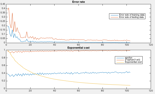
How the AdaBoost is iteratively trained can be seen in the figure below. First, the error rate, the ratio between the number of misclassified samples and the total number of samples, for both the training and testing samples, are plotted as the iteration progresses (top). Also, the weighted error $\varepsilon_t$, the exponential costs $E_t$, and the ratio $E_{t+1}/E_t=2\sqrt{\varepsilon_t(1-\varepsilon_t)}$ are all plotted (bottom). We see that $\varepsilon_t<0.5$ and $E_{t+1}/E_t<1$ for all steps, and the exponential cost $E_t$ attenuates exponentially towards zero.

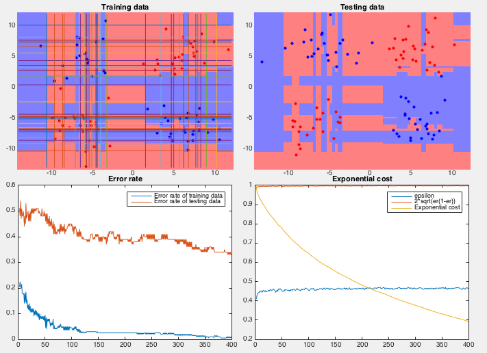
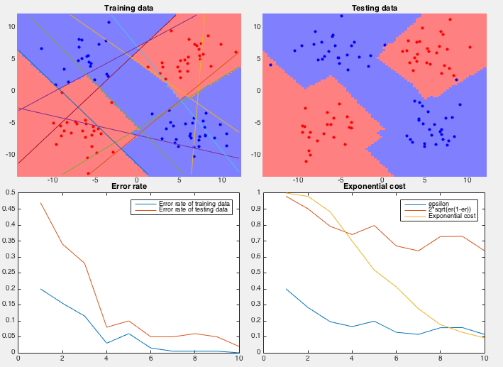
Example 2 In this dataset, 100 training samples of two classes (50 each) forms four clusters arranged in the 2-D space as an XOR pattern as shown figure (top-left), and 100 testing samples of the same distribution are classified by the AbaBoost algorithm trained by both the coordinate descent and PCA methods.

We see that the coordinate descent method performs very poorly in both the slow convergence (more than 400 iterations) during training and high classification error rate (more than 1/3) during testing. The partitioning of the 2-D space is an obvious over fitting of the training set instead of reflecting the actual distribution of the two classes (four clusters). On the other hand, the PCA method converges quickly (10 iterations) and classifies the testing samples with very low error rate. The space is clearly partitioned into two regions corresponding to the two classes.