Application to Image Data

The KLT can be applied to a set of $N$ images for various purposes such as data compression and feature extraction. There are two alternative ways to carry out the KLT on the $N$ images each containing $K$ pixels, depending on how the random vector ${\bf x}$ is defined based on the image data which can be represented in the form of an $N\times K$ 2-D array.

• A $K$-dimensional vector ${\bf x}_n$ can be formed by all $K$ pixels (by concatenating the rows or columns) of each of the $N$ images. These $N$ vectors each for one of the $N$ images are represented by a $K\times N$ data array ${\bf X}=[{\bf x}_1,\cdots,{\bf x}_N]$, and treated as the samples of a K-dimensional random vector ${\bf x}$, its covariance matrix can be estimated (assuming with zero mean) as:

  $${\bf\Sigma}=\frac{1}{N} \sum_{n=1}^N{\bf x}_n{\bf x}_n^T =\frac{1... ...N^T\end{array}\right] =\frac{1}{N} \left( {\bf X} {\bf X}^T \right)_{K\times K}$$ (86)

• An $N$-dimensional vector can be formed by the pixels at the same position (in the $i$th row and $j$th column of the image array) from all $N$ images. There are $K$ such vectors each for one of the $K$ pixels in the images. These vectors are the rows of the ${\bf X}$ defined above, or the columns of ${\bf X}^T$. The covariance matrix of these $N$ dimensional vectors can be estimated as:

  $${\bf\Sigma}'=\frac{1}{K} \left( {\bf X}^T{\bf X}\right)_{N\times N}.$$ (87)

As shown previously, these two different covariance matrices share the same eigenvalues. The eigenequations for ${\bf X}^T{\bf X}$ and ${\bf X}^T{\bf X}$ (with the constant coefficients $1/K$ and $1/N$ neglected) are:

$${\bf X}^T{\bf X}{\bf v}=\lambda{\bf v}, \;\;\;\;\;\;\;\;\;\;\;\;\;\;\;\;\;\; {\bf X}{\bf X}^T{\bf u}=\mu{\bf u}.$$ (88)

Pre-multiplying ${\bf X}^T$ on both sides of the second equation we get

$${\bf X}^T{\bf X} [{\bf X}^T{\bf u}]=\mu [{\bf X}^T{\bf u}].$$ (89)

which is actually the first eigenequation with the same eigenvalue $\mu=\lambda$ and eigenvector ${\bf v}={\bf X}^T{\bf u}$ when normalized. The two covariance matrices ${\bf\Sigma}$ and ${\bf\Sigma}'$ have the same rank $R=\min(N,K)$ (if ${\bf X}$ is not degenerate) and therefore the same number of non-zero eigenvalues. Consequently, the KLT can be carried out based on either matrix with the same effects in terms of the signal decorrelation and energy compaction. As the number of pixels in the image is typically much greater than the number of images, $K>N$, we will take the second approach above to treat the pixels in the same position in all $N$ images as a sample of an $N$-dimensional random signal vector and carry out the KLT based on the $N\times N$ covariance matrix $\hat{{\bf\Sigma}}$.

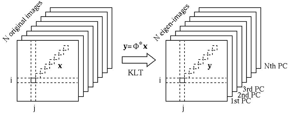
We can now carry out the KLT to each of the $K$ $N$-dimensianl vectors ${\bf x}$ corresponding to each pixel of the $N$ images to obtain another $N$-dimensional vector ${\bf y}={\bf v}^*{\bf x}$ for the same pixel of a set of $N$ eigen-images, as shown below. After the KLT, most of the energy/information contained in the $N$ images, representing the variations among all $N$ images, is concentrated in the first few eigen-images corresponding to the greatest eigenvalues, while the remaining eigen-images can be omitted without losing much energy/information. This is the foundation for various KLT-based image compression and feature extraction algorithms. The subsequent operations such as image recognition and classification can all be carried out in a much lower dimensional space.

We now consider some of such applications.

• Remote sensing data compression

  In remote sensing, images of the surface of either the Earth or other planets such as Mars are taken by a multispectral camera system on board satellite, for various studies (e.g., geology, geography, etc.). The camera system has an array of $N$ sensors, typically a few tens or even over a hundred, each sensitive to a different wavelength band in the visible and infrared range of the electromagnetic spectrum. Depending on the number of sensors, the data are referred to as either multi or hyper-spectral images.

  These sensors will produce a set of $N$ images covering the same surface area on the ground. For the same position in these images, there are $N$ pixel values each from one wavelength band representing the spectral profile that characterizes the material on the surface area corresponding to the pixel. A typical application of the multi or hyper-spectral image data is to classify the pixels into different types of materials (different types of rocks, vegetations, polutions, etc.). When $N$ is large, KLT can be used to reduce the dimensionality without loss of much information. Specifically, we consider the $N$ values associated with each pixel form an N-dimensional random vector, and then carry out KLT to reduce its dimensionality. All classification can be carried out in this low dimensional space, thereby significantly reducing the computational complexity.

  

  

• Video image compression

  A sequence of $N=8$ frames of a video of a moving escalator and their eigen-images are shown respectively in the upper and lower parts of the figure below.

  

  It is interesting to observe that the first eigen-image corresponding to the greatest eigenvalue (left panel of the third row of the figure) represents mostly the static scene of the image frames representing the main variations in the image (carrying most of the energy), while the subsequent eigen-images represent mostly the motion in the video, the variation between the frames. For example, the motion of the people riding on the escalator is mostly reflected by the first few eigen-images following the first one, while the motion of the escalator stairs is mostly reflected in the subsequent eigen-images.

  The $8\times 8$ covariance matrix and the energy distribution among the eight components plot before and after the KLT are shown below.

  

  We see that due to the spatial correlation between nearby pixels, the covariance matrix before the KLT (left) can be modeled by the squared exponental function, while the covariance matrix after the KLT (middle) is completely decorrelated and the energy is highly compacted into a small number of principal components (here the first component), as also clearly shown in the comparison of the energy distribution before and after the KLT (right).

• Eigenface and face recognition

  Twenty images of faces ($N=20$):

  

  The eigen-images after KLT:

  

  Percentage of energy contained in the

  components	1	2	3	4	5	6	7	8	9	10	11	12	13	14	15	16	17	18	19	20
  percentage energy	48.5	11.6	6.1	4.6	3.8	3.7	2.6	2.5	1.9	1.9	1.8	1.6	1.5	1.4	1.3	1.2	1.1	1.1	0.9	0.8
  accumulative energy	48.5	60.1	66.2	70.8	74.6	78.3	81.0	83.5	85.4	87.3	89.	90.7	92.2	93.6	94.9	96.1	97.2	98.2	99.2	100.0

  Reconstructed faces using 95% of the total information (15 out of 20 components):

  

• Hand-written number recognition

  The goal here is to recognize hand-written number from 0 to 9 in an image, as those in the figure below, containing $N=2240$ samples for the $K=10$ numbers. Each sample in the $16\times 16$ image can be represented by a $d=16\times 16=256$ dimensional vector by concatenating all columns (or rows) of the image. The KLT can be carried out to significantlly reduce the dimensionality of the vectors from $d=256$ to some $d'\ll d$, based on either the covariance matrix ${\bf\Sigma}_x={\bf S}_T$ of all $N=2240$ sample vectors representing the over all distribution of these data points, or the between-class scatter matrix ${\bf S}_B$ previously considered representing the separability of the ten classes.

  Specifically, we use the eigenvectors corresponding to the $d'$ greatest eigenvalues of the covariance matrix or the between-class scatter matrix to form a $d'$ by $d$ transform matrix. After the KLT transform by the data, certain classification algorithm can be carried out in the much reduced d' dimensional space.

  

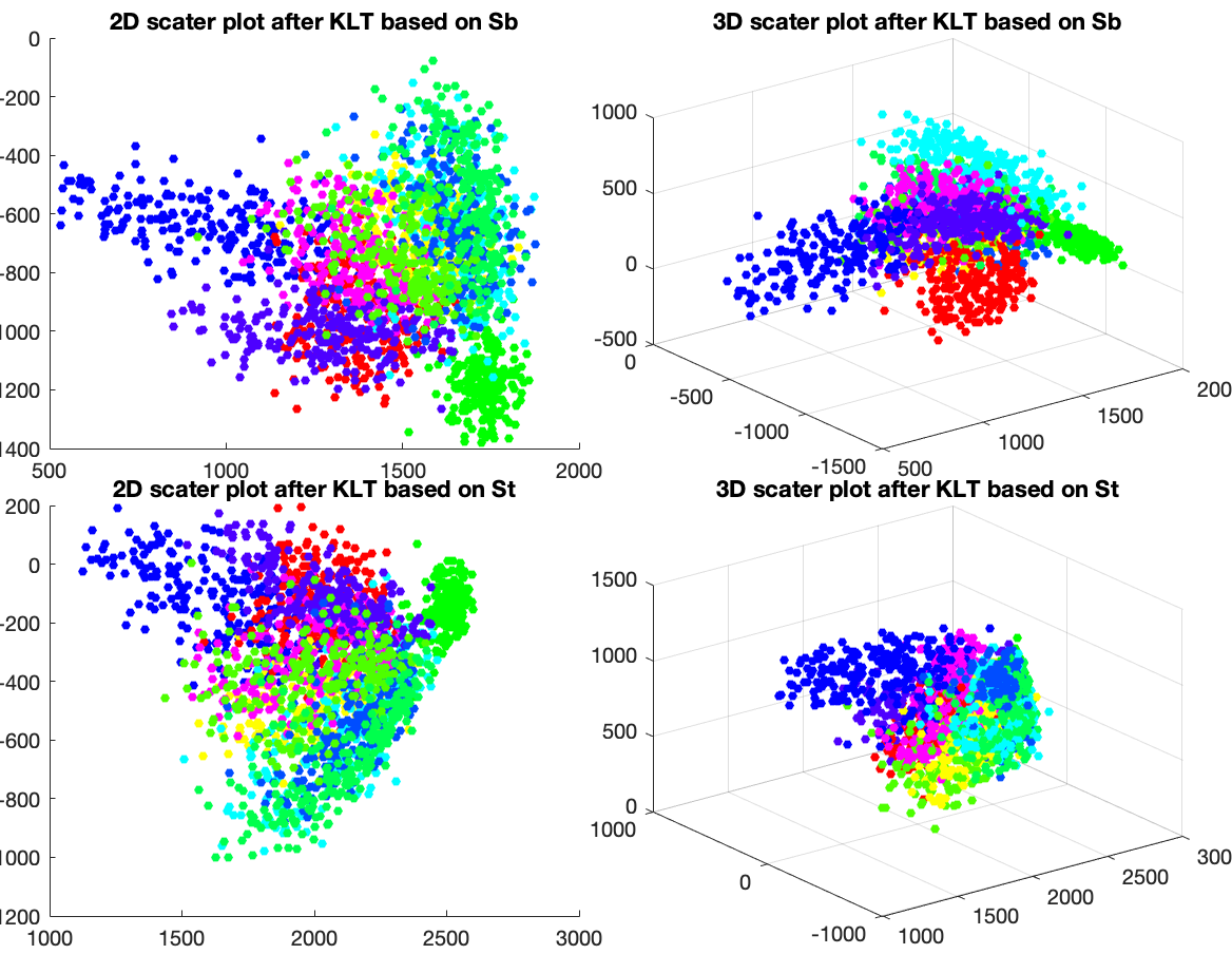
  The energy distribution over all $d=256$ signal components is plotted below for the original signal (top), after the KLT based on ${\bf S}_B$ (middle), and after the KLT based on ${\bf S}_T$.

  

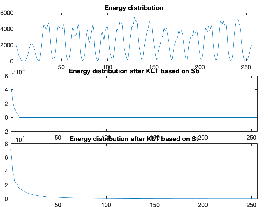
  For the KLT based on ${\bf S}_T$ with rank $N-1$, $d'=79$ components are needed to keep 95.1% of the total energy, in comparison to the KTL based on ${\bf S}_B$ with rank $\rank({\bf S}_B)=K-1=9$, requiring are only $d'=9$ principal components corresponding to the same number of non-zero eigenvalues of ${\bf S}_B$ to keep 100% of the total energy representing the separability information. The percentage energy conteined in these non-zero eigenvalues are: $28.6\%,\; 22.7\%,\; 14.4\%,\; 10.9\%,\;7.1\%,\; 7.0\%,\; 3.8\%,\; 3.2\%,\; 2.4\%$.

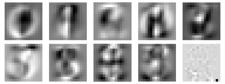
  The corresponding $d=256$ dimensional eigenvectors can be visualized when converted to $16\times 16$ eigenimages, representing the basis by which any original images can be represented as a linear combination of such eigenimages, as shown in the figure below. The 10th eigenimage corresponding to a zero eigenvalue contains only some random noise.

  

  If we only keep the first two or three principal components (corresponding to the greatest eigenvalues) after the KLT, the dataset can be visualized as shown in the figure below. The sample points in each of the ten different classes are color-coded. It can be seen that even when the dimensions are much reduced from $N=256$ to $d=3$ or even $d=2$, it is still possible to separate the ten classes reasonably well.