Comparison with Other Orthogonal Transforms

Here we compare the KLT, in terms of signal decorrelation and energy compaction, with other orthogonal transforms such as discrete cosine transform (DCT) and Fourier transform (DFT), as well as identity transform IT (no transform), based on two images of cloud and sand as shown below.

We treat each colume of the image as an observation (instantiation) of a 1-D random vector ${\bf x}$, and apply an orthogonal transforms ${\bf y}={\bf A}^T{\bf x}$ to ${\bf x}$ based on the covariance matrix ${\bf\Sigma_x}$, and compare the corresponding covariance matrices ${\bf\Sigma}_y$ after the transform to see how well each transform decorrelates the signal and compacts its energy.

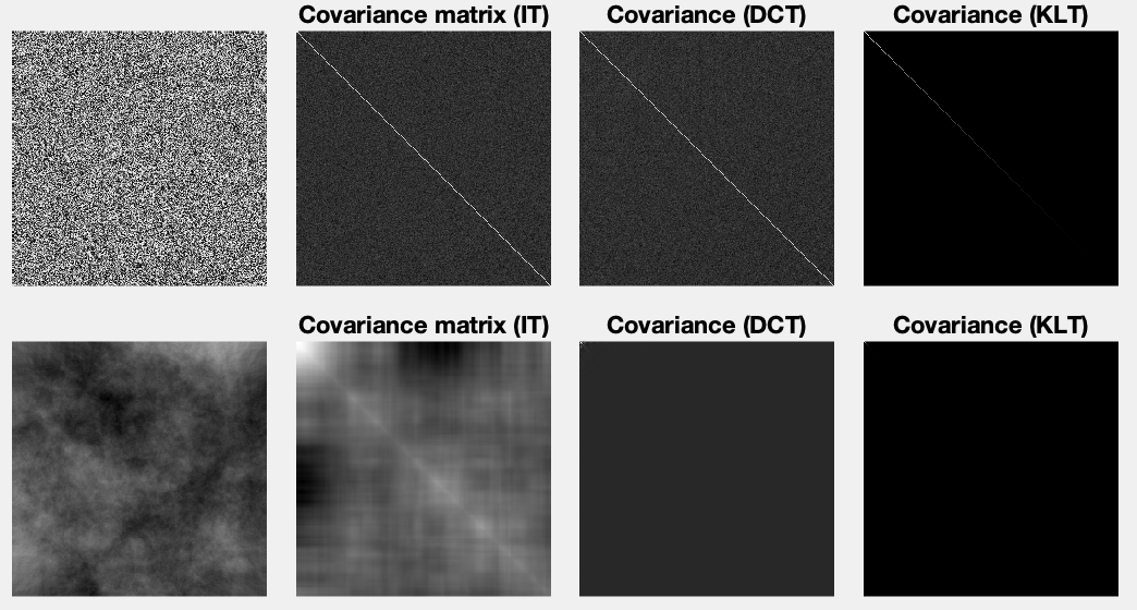
The figure below shows the original images (left) and the covariance matrices in image form (pixel values proportional to the values in the covariance matrix) after three orthogonal transforms of IT, DCT, and KLT.

• Sand image

  In the second panel showing the covariance after IT, the off-diagonal pixels are dark, indicating the pixels in the original image are not hithly correlated at all. In the third panel, the covariance after DCT looks similar to that before the transform, indicating that the DCT has little effect in terms of signal decorrelation and energy compaction. Finally, in the right-most panel showing the covariance after KLT, all off diagonal elements are zero, i.e., the signal components are completely decorrelated.

• Cloud image

  In the second panel for the covariance after IT, there exist some bright areas off the diagonal, indicating that many signal components close to each other are highly correlated. In the third panel for the covariance after DCT, the values of the off diagonal elements are significantly reduced, indicating that the signal components are significantly decorrelated. Finally, in the right-most panel showing the covariance after KLT, all off diagonal elements are zero, i.e., the signal components are completely decorrelated.

The effect of energy redistribution and compaction of these different transforms are also shown in the figure below, where the variances of signal components are sorted and plotted.

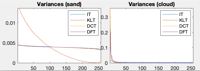
We see that due to the physical nature of the clouds and sand grains, the textures in the corresponding images are very different. In the cloud image, the neighboring pixels are highly correlated, while in the sand image, they are not much correlated at all. Correspondingly, the DCT can effectively decorrelate the cloud image, but much less so in the sand image. But in either case, whether the pixels in the image are highly correlated or not, the KLT can always completely decorrelate the signal and optimally compact the energy.

The table below further demonstrate the effect of energy compaction quantitatively in terms of the number of components out of the total of 256 components needed after the transform in order to keep a certain percentage of the total dynamic energy (information). For example, if it is desired to keep 95% of the total energy contained in the original signal, 230 components are needed with no transform, 22 are needed after DCT, and only 13 are needed after KLT. Note that DCT's performance is reasonably close to that of the optimal KLT in this case.

$$\begin{array}{l\vert\vert r\vert r\vert r\vert r} \hline \mbo... ... & 256 \\ \hline KLT: & 7 & 13 & 55 & 256 \\ \hline \end{array}$$ (85)

Although KLT is optimal in terms of signal decorrelation and energy compaction, it is not as convenient as other transforms for two reasons. First, the KLT is data-specific, i.e., the transform matrix is the eigenvector matrix of the covariance matrix of the dataset, which needs to be estimated based on sufficient amount of data samples, while all other orthogonal transforms are data indepenent. Seond, the computational cost of the KLT is significantly higher than that of other transforms, due to the $O(d^3)$ complexity for solving the eigenvalue problem of the $d \times d$ matrix covairance matrix ${\bf\Sigma}_x$, while for most other popular orthogonal transforms fast algorithm exist with $O(d\log_2 d)$ complexity instead of $O(d^2)$ required by the KLT.