Classical Multidimensional Scaling

The goal of multidimensional scaling (MDS) is to reduce the dimensionality of the dataset representing a set of $N$ objects of interest, each described by a set of $d$ features and represented as a vector ${\bf x}=[x_1,\cdots,x_d]^T$ in a d-dimensional space, while the pairwise similarity relationship between any two of these objects are preserved. MDS can be used to visualize datasets in a high dimensional space. Specially, here we consider the classical MDS (cMDS), also known as principal coordinates analysis (PCoA), as one of the methods in MDS. Here is an example visualizing the US House of Representatives based on their voting patterns.

Specifically, we represent the pairwise similarity of a set of $N$ objects ${\bf X}=[{\bf x}_1,\cdots,{\bf x}_N]$ by the $N\times N$ similarity matrix ${\bf D}_x=[\;d^x_{ij}\;]$, of which the ij-th component $d^x_{ij}$ is certain measurement of the similarity between ${\bf x}_i$ and ${\bf x}_j$. The goal is to map the dataset ${\bf X}$ in the d-dimensional space into ${\bf Y}=[{\bf y}_1,\cdots,{\bf y}_N]$ in a lower d'-dimensional space, in which the similarity matrix ${\bf D}_x$ is optimally approximated by ${\bf D}_y=[\; d^y_{ij} ]$. When $d'\le 3$, these data points in ${\bf Y}$ can be visualized. MDS can be considered as a method for dimension reduction. In some cases only the pairwise similarities $d^x_{ij}\;(i,j=1,\cdots,N)$ are given, while the $N$ objects in ${\bf X}$ are not explicitly given, and the dimensionality $d$ may be unknown.

We assume the given pairwise similarity is the Euclidean distance $d_{ij}=\vert\vert{\bf x}_i-{\bf x}_j\vert\vert _2$ between ${\bf x}_i$ and ${\bf x}_j$:

$$d^2_{ij}=\vert\vert{\bf x}_i-{\bf x}_j\vert\vert^2 =({\bf x}_i-{\... ...}_i-{\bf x}_j) ={\bf x}_i^T{\bf x}_i-2{\bf x}_i^T{\bf x}_j+{\bf x}_j^T{\bf x}_j$$ (170)

and get

$${\bf D}_x^2=\left[\begin{array}{ccc} & & \\ & d^2_{ij} & \\ & & ... ... &\\ & & \end{array}\right]_{N\times N} ={\bf X}_r-2{\bf X}^T{\bf X}+{\bf X}_c$$ (171)

where

$${\bf X}_r = \left[\begin{array}{ccc}\vert\vert{\bf x}_1\vert\vert^2&\cdots&\v... ...ert\vert^2&\cdots&\vert\vert{\bf x}_N\vert\vert^2\end{array}\right]={\bf X}_c^T$$

$${\bf X}^T{\bf X} = \left[\begin{array}{c}{\bf x_1}^T\\ \vdots\\ {\bf x}_N^T\end{arra... ...ts&\vdots\\ {\bf x}_N^T{\bf x}_1&\cdots&{\bf x}_N^T{\bf x}_N\end{array}\right]$$ (172)

Our goal is to find ${\bf Y}=[{\bf y}_1,\cdots,{\bf y}_N]$ in a lower dimensional space so that its pairwise similarity matrix ${\bf D}_y$ matches ${\bf D}_x$ optimally, in the sense that the following objective function is minimized:

$$J({\bf Y})=\vert\vert {\bf D}^2_y-{\bf D}_x^2\vert\vert$$ (173)

We note that such a solution ${\bf Y}$ is not unique, as any translated version of ${\bf Y}$ has the same pairwise similarity matrix and is also a solution. We therefore seek to find a unique solution ${\bf Y}$ in which all data points are centralized, i.e, the mean of all points in ${\bf Y}$ is zero:

$$\bar{\bf y}=\frac{1}{N}\sum_{n=1}^N {\bf y}_n={\bf0}$$ (174)

To do so, we introduce an $N\times N$ symmetric centering matrix ${\bf C}={\bf I}-{\bf 1}/N={\bf C}^T$, where ${\bf 1}={\bf ee}^T$ is an $N\times N$ matrix with all components equal 1. Premultiplying ${\bf C}$ to a column vector ${\bf a}=[a_1,\cdots,a_N]^T$ removes the mean $\bar{a}=\sum_{i=1}^N a_i/N$ of ${\bf a}$ from each of its component:

$${\bf Ca} ={\bf Ia}-\frac{1}{N}{\bf 1}{\bf a} =\left[\begin{array}... ...t] =\left[\begin{array}{c}a_1-\bar{a}\\ \vdots\\ a_N-\bar{a} \end{array}\right]$$ (175)

Taking transpose of the equation above, we get

$$({\bf Ca})^T={\bf a}^T{\bf C}=[a_1-\bar{a},\cdots,a_N-\bar{a}]$$ (176)

i.e., postmultiplying ${\bf C}$ to a row vector ${\bf a}^T=[a_1,\cdots,a_N]$ removes the mean $\bar{a}$ from each of its component.

We can now postmultiply ${\bf C}$ to ${\bf X}$ to remove the mean of each row of ${\bf X}$:

$${\bf XC}=[{\bf x}_1,\cdots,{\bf x}_N]{\bf C} =[\bar{\bf x}_1,\cdots,\bar{\bf x}_N]=\bar{\bf X}$$ (177)

i.e., the nth column becomes:

$$\bar{\bf x}_n={\bf x}_n-\bar{\bf x},\;\;\;\; \;\;\;\; \bar{\bf x}=\frac{1}{N}\sum_{n=1}^N{\bf x}_n$$ (178)

and premultiply ${\bf C}$ to ${\bf X}^T$ to remove the mean of each column of ${\bf X}^T$:

$${\bf CX}^T=\bar{\bf X}^T$$ (179)

We further apply double centering to ${\bf D}_x^2$ by pre and post-multiplying ${\bf C}$ and get:

$${\bf CD}_x^2{\bf C} = {\bf C}\left( {\bf X}_r-2{\bf X}^T{\bf X}+{\bf X}_c \right) {\bf ... ...f CX}_r{\bf C} -2{\bf C}\left({\bf X}^T{\bf X}\right){\bf C} +{\bf CX}_c{\bf C}$$

$$= -2{\bf C}\left({\bf X}^T{\bf X}\right){\bf C} =-2\left( {\bf X}{\bf C} \right)^T\left( {\bf X}{\bf C} \right) =-2\bar{\bf X}^T\bar{\bf X}$$

Note that the first term ${\bf CX}_r{\bf C}={\bf C}({\bf X}_r{\bf C})={\bf C0}={\bf0}$, as all components of each row of ${\bf X}_r$ are the same as their mean, and removing the mean results in a zero row vector, ${\bf X}_r{\bf C}={\bf0}$; and the last term ${\bf CX}_c{\bf C}=({\bf CX}_c){\bf C}={\bf0C}={\bf0}$, as all components of each column of ${\bf X}_c$ are the same as their mean, and removing the mean results in a zero column vector.

Now the similarity matrix ${\bf D}_x^2$ of all centralized data points in $\bar{\bf X}$ with zoero mean can be represented by the Gram matrix of $\bar{\bf X}$:

$${\bf G}_{\bar{x}}=\bar{\bf X}^T\bar{\bf X}=-\frac{1}{2}{\bf CD}_x^2{\bf C}$$ (180)

We further assume all data points in ${\bf Y}$ are also centeralized with zero mean and their corresponding similarity matrix is also represented by ${\bf G}_{\bar{y}}$, then the objective function can be expressed as:

$$J({\bf Y})=\vert\vert {\bf G}_{\bar{y}}-{\bf G}_{\bar{x}} \vert\vert =\vert\vert \bar{\bf Y}^T\bar{\bf Y}-{\bf G}_{\bar{x}} \vert\vert$$ (181)

To find $\bar{\bf Y}$ that minimizes $J({\bf Y})$, we first consider the equation $\bar{\bf Y}^T\bar{\bf Y}-{\bf G}_{\bar{x}}={\bf0}$ so that $J({\bf Y})=0$. In other words, we desire to express ${\bf G}_{\bar{x}}$ as the inner product of some matrix with itself. To do so, we carry out eigenvalue decomposition of ${\bf G}_x$ to find its eigenvalue matrix ${\bf\Lambda}$ and the orthogonal eigenvector matrix ${\bf V}$ satisfying ${\bf G}_x{\bf V}={\bf V}{\bf\Lambda}$, i.e.,

$${\bf G}_{\bar{x}} = {\bf V}{\bf\Lambda}{\bf V}^{-1} ={\bf V}{\bf\Lambda}{\bf V}^T=[{\... ...ght] \left[\begin{array}{c}{\bf v}_1^T\\ \vdots\\ {\bf v}_N^T\end{array}\right]$$

$$= \left({\bf V}{\bf\Lambda}^{1/2}\right)\,\left({\bf\Lambda}^{1/2}{... ...ft({\bf\Lambda}^{1/2}{\bf V}^T\right)^T\left({\bf\Lambda}^{1/2}{\bf V}^T\right)$$

Note that as ${\bf G}_{\bar{x}}$ is symmetric, the eigenvalues are real and the eigenvectors are orthogonal, i.e., ${\bf V}^T={\bf V}^{_1}$ is is orthogonal matrix. Now we can find the desired ${\bf Y}$ as:

$${\bf Y}={\bf\Lambda}^{1/2}{\bf V}^T =\left[\begin{array}{ccc}\sqr... ...lambda_1}{\bf v}_1^T\\ \vdots\\ \sqrt{\lambda_N}{\bf v}_N^T\end{array} \right]$$ (182)

Each column ${\bf y}_i$ in ${\bf Y}=[{\bf y}_1,\cdots,{\bf y}_N]$ is an N-D vector. If all $N$ dimensions of these ${\bf y}_n$ are used, ${\bf Y}^T{\bf Y}={\bf G}_x$ and $J({\bf Y}=0$. To reduce the dimensionality to $d'<d$, we construct ${\bf Y}'$ by the first $d'$ rows of ${\bf Y}$ corresponding to the $d'$ greatest eigenvalues of $\lambda_1\ge\cdots\ge\lambda_{d'}\ge\cdots\ge\lambda_N$ and their corresponding eigenvectors ${\bf v}_1,\cdots,{\bf v}_{d'}$. The error is:

$$J({\bf Y}')=\vert\vert{\bf Y}'^T{\bf Y}'-{\bf Y}^T{\bf Y}\vert\ve... ...bf v}^T\vert\vert =\vert\vert\sum_{i=d'}^N\lambda_i{\bf v}_i{\bf v}^T\vert\vert$$ (183)

In summary, here is the PCoA algorithm:

• Given the pairwise similarity, an $N\times N$ matrix ${\bf D}_x=[\;d_{ij}\;]$, construct the squared proximity matrix ${\bf D}^2_x=[\;d^2_{ij}\;]$;
• Apply double centering to get ${\bf G}_x=-{\bf C}{\bf D}^2_x{\bf C}/2$;
• Find the $d'$ greatest eigenvalues $\lambda_1,\cdots,\lambda_{d'}$ of ${\bf G}_x$, and the corresponding eigenvectors ${\bf v}_1,\cdots,{\bf v}_{d'}$;
• Get the map

  $${\bf Y}_{d'\times N}={\bf\Lambda}_{d'}^{1/2}{\bf V}_{d'} =\left[\... ..._1}{\bf v}_1^T\\ \vdots\\ \sqrt{\lambda_{d'}}{\bf v}_{d'}^T\end{array} \right]$$ (184)

The Matlab functions for the PCA and PCoA are listed below:

function Y=PCA(X)
    [V D]=eig(cov(X'));         % solve eigenequation for covariance of data
    [d idx]=sort(diag(D),'descend');    % sort eigenvalues in descend order
    V=V(:,idx);                         % reorder eigenvectors
    Y=V'*X;                             % carry out KLT
end


function Y=PCoA(X)
    N=size(X,2);
    D=zeros(N);                         % pairwise similarity matrix
    C=eye(N)-ones(N)/N;                 % centering matrix
    for i=1:N
        for j=1:N
            D(i,j)=(norm(X(:,i)-X(:,j)))^2;
        end
    end
    B=-C*D*C/2;
    [V D]=eig(B);                       % solve eigenequation for matrix B
    [d idx]=sort(diag(D),'descend');    % sort eigenvalues in descend order
    V=V(:,idx);                         % reorder eigenvectors
    Y=sqrt(D)*V';                       % carry out PCoA
end

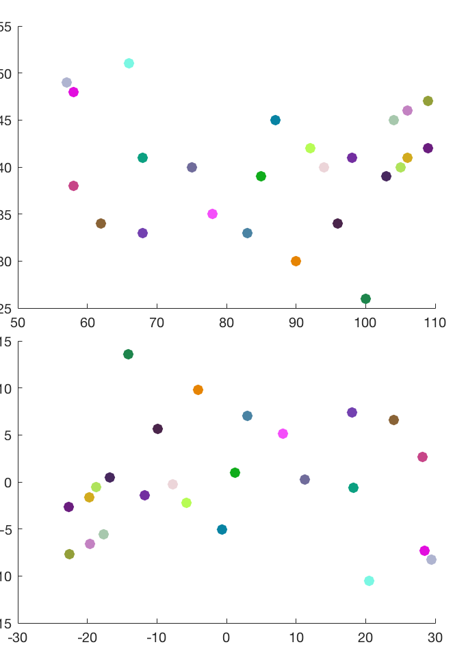
Example 1:

In the figure below, the top panel shows the locations of some major cities in North America, and the bottom panel shows the reconstructed city locations based on the pairwise distance of these cities. Note that the reconstructed map is a rotated and centralized version of the original map.

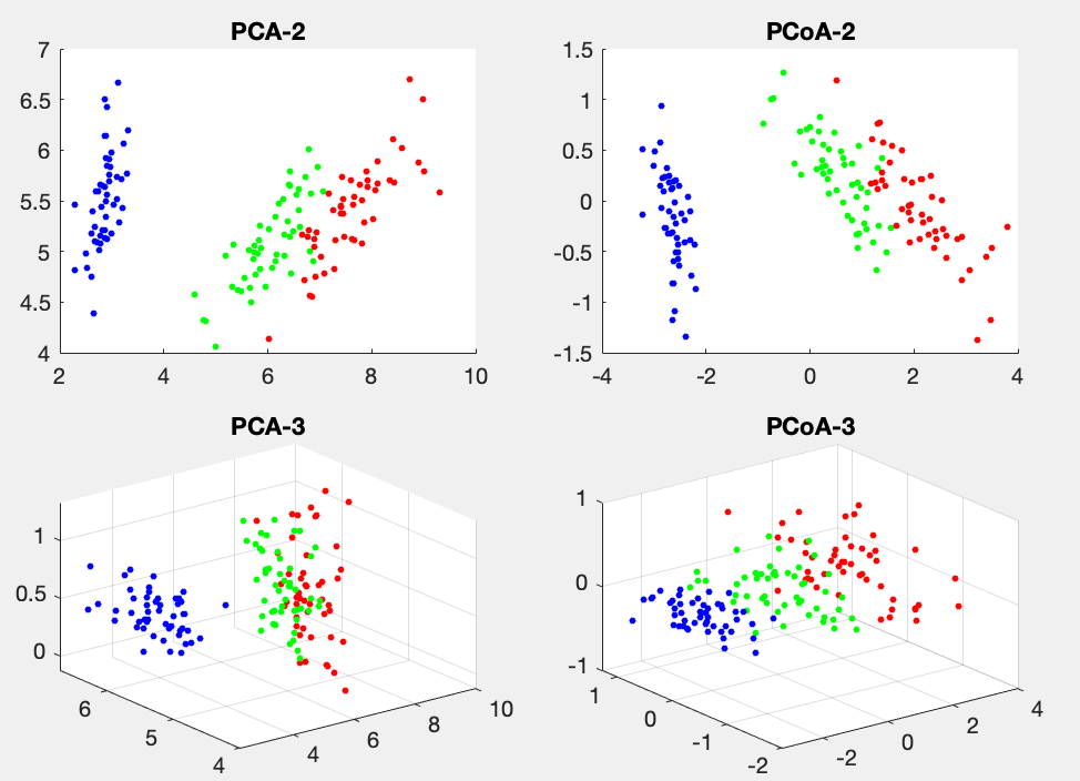
Example 2:

Both PCA and PCoA are applied to the Iris dataset of 150 4-D data points, and the figure below shows the data points in 2-D and 3-D spaces corresponding to the first 2 and 3 eigenvalues.

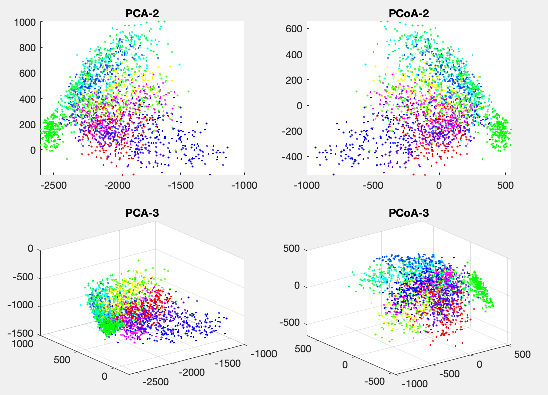
Example 3:

Both PCA and PCoA are applied to the dataset of handwritten numbers of 2240 256-D data points, and the figure below shows the data points in 2-D and 3-D spaces corresponding to the first 2 and 3 eigenvalues.