Probabilistic PCA

The method of probabilistic PCA (PPCA) can be considered as a special case of factor analysis based on the model ${\bf x}={\bf Wz}+{\bf e}$, when the random noise ${\bf e}$ is assumed to have an isotropic normal distributions with covariance matrix ${\bf\Psi}=\varepsilon{\bf I}$. More specially, if we further let $\varepsilon\rightarrow 0$ approach zero, the iteration of the EM algorithm for the PPCA becomes extremely simple, as we will see below.

Same as in Eqs. (125) and (127) for FA, here we also have the normal distribution of both ${\bf z}$ and ${\bf e}$:

$$p({\bf z})={\cal N}({\bf0},{\bf I}), \;\;\;\;\;\;\;\;\;\;\;\;\;\;\; p({\bf e})={\cal N}({\bf0},\varepsilon{\bf I})$$ (150)

and the normal distribution of the observed data ${\bf x}={\bf Wz}+{\bf e}$, same as in Eq. (131):

$$p({\bf x})={\cal N}({\bf0},{\bf WW}^T+\varepsilon{\bf I})$$ (151)

The goal here is to estimate $\varepsilon$ and ${\bf W}$ as the model parameter, based on the observed data dataset ${\bf X}=[{\bf x}_1,\cdots,{\bf x}_N]$.

Now Eqs. (137) through (139) are rewritten as:

$$\left\{\begin{array}{l} {\bf m}_{z\vert x_n}=E_{z\vert x_n}({\bf ... ...gma}_{z\vert x_n}=Cov_{z\vert x_n}({\bf z})={\bf I}-{\bf BW} \end{array}\right.$$ (152)

$${\bf B}={\bf W}^T({\bf WW}^T+\varepsilon{\bf I})^{-1}$$ (153)

$$({\bf WW}^T+\varepsilon{\bf I})^{-1} =\varepsilon^{-1}{\bf I}-\varepsilon^{-1}{\bf W}(\varepsilon{\bf I}+{\bf W}^T{\bf W})^{-1}{\bf W}^T$$ (154)

The two steps of the EM algorithm become:

• E-step: Get the expectation of the log likelihood by replacing ${\bf\Psi}$ in Eq. (142) by $\varepsilon{\bf I}$:

  $$Q =-\frac{dN}{2}\log\varepsilon-\frac{1}{2\varepsilon} \sum_{n=1}... ... {\bf x}_n^T{\bf x}_n -2{\bf x}_n^T{\bf Wz} +{\bf z}^T{\bf W}^T{\bf Wz} \right]$$ (155)

• M-step: Find the optimal model parameters ${\bf W}$ and $\varepsilon$ that maximize the expectation of the log likelihood $Q$ above, by setting the derivative of $Q$ with respect to the parameters to zero and solve the resulting equations. For ${\bf W}$, the result is the same as Eq. (145):

  $${\bf W}_{new}=\left(\sum_{n=1}^N {\bf x}_n E_{z\vert x_n}[{\bf z}^T]\right)\; \left(\sum_{n=1}^N E_{z\vert x_n}[{\bf zz}^T] \right)^{-1}$$ (156)

  where

  $$\left\{\begin{array}{lll} E_{z\vert x_n}[{\bf z}]&=&{\bf m}_{z\ve... ...gma}_{z\vert x_n}+{\bf m}_{z\vert x_n}{\bf m}_{z\vert x_n}^T \end{array}\right.$$ (157)

  To find $\varepsilon$, we solve the equation

  $$\frac{\partial Q}{\partial \varepsilon} =-\frac{dN}{2\varepsilon}... ...f x}_n^T{\bf x}_n -2{\bf x}_n^T {\bf Wz} + {\bf z}^T{\bf W}^T{\bf Wz} \right]=0$$ (158)

  and get
  

  $$\varepsilon = \frac{1}{dN} \sum_{n=1}^N \left[ {\bf x}_n^T{\bf x}_n -2{\bf x}_n... ...\vert x_n}({\bf z}) + tr ({\bf W}^T E_{z\vert x_n} ({\bf zz}^T){\bf W}) \right]$$

  $$= \frac{1}{dN} \sum_{n=1}^N \left[ \vert\vert{\bf x}_n\vert\vert^2 ... ...T){\bf W}^T{\bf x}_n + tr (E_{z\vert x_n} ({\bf zz}^T){\bf W}^T{\bf W}) \right]$$ (159)

  
  where we have used the fact that ${\bf a}^T{\bf b}=tr({\bf ab}^T)$.

In summary, here are the steps in the EM algorithm for PPCA:

1. Initialize parameters ${\bf\theta}_{old}=\{{\bf W}_{old},\varepsilon_{old}\}$;
2. E-step: Based on ${\bf\theta}_{old}$, find ${\bf m}_{z\vert x_n}$ and ${\bf\Sigma}_{z\vert x_n}$ in Eq. (152), and $E_{z\vert x_n}({\bf z})$ and $E_{z\vert x_n}({\bf zz}^T)$ in Eq. (157);
3. M-step: Find ${\bf\theta}_{new}=\{{\bf W}_{new},\varepsilon_{new}\}$ by evaluating Eqs. (156) and (159);
4. Terminate if convergence cretierion is satisfied, otherwise replace $\theta_{old}$ by $\theta_{new}$ and return to step 2.

Specially, if we further assume $\varepsilon\rightarrow 0$ and the latent variables in ${\bf z}$ are deterministic, i.e., $E_{z\vert x}({\bf z})={\bf z}$. At the limit where $\varepsilon=0$, ${\bf x}$ is simply a linear combination of the latent variables in ${\bf z}$:

$${\bf x}={\bf Wz}+\varepsilon{\bf I} \;\;\stackrel{\varepsilon\rig... ...{array}{c}z_1\\ \vdots\\ z_{d'}\end{array}\right] =\sum_{i=1}^{d'} z_i{\bf w}_i$$ (160)

Comparing this expression of ${\bf x}$ with Eq. (81)

$${\bf x}={\bf V}'{\bf y}=\sum_{i=1}^{d'} y_i{\bf v}_i$$ (161)

we see that the column vectors in ${\bf W}=[{\bf w}_1,\cdots,{\bf w}_{d'}]$ for the PPCA are similar to the column vectors of ${\bf V}$ , the eigenvector matrix of ${\bf\Sigma}_x$, in the linear PCA, as both of them can be viewed as the principal directions, an alternative set of basis vectors that also span the same d-dimensional feature space in which ${\bf x}$ resides. When ${\bf x}$ is expressed as a linear combination of these basis vectors, it can be approximated by only $d'<d$ of the $d$ such basis vectors weighted by the $d'$ principal components in ${\bf y}=[y_1,\cdots,y_{d'}]^T$ in linear PCA, or the $d'$ factors in ${\bf z}=[z_1,\cdots,z_{d'}]^T$ in PPCA.

Here are the two EM steps for the PPCA:

• E-step: If $\varepsilon\rightarrow 0$, Eq. (152) can be written as:
  

  $${\bf m}_{z\vert x_n} = E_{z\vert x_n}({\bf z})={\bf z}_n={\bf Bx}_n ={\bf W}^T({\bf WW}^T+\varepsilon{\bf I})^{-1}{\bf x}_n$$

  $$\stackrel{\varepsilon\rightarrow 0}{\Longrightarrow} {\bf W}^T({\bf WW}^T)^{-1}{\bf x}_n\;\;\;\;\;\;(n=1,\cdots,N)$$ (162)

  
  All $N$ such equations can be written in matrix form as

  $${\bf Z}=[{\bf z}_1,\cdots,{\bf z}_n] ={\bf W}^T({\bf WW}^T)^{-1}[{\bf x}_1,\cdots,{\bf x}_N] ={\bf W}^T({\bf WW}^T)^{-1}{\bf X}$$ (163)

  As ${\bf W}$ is a $d\times d'$ matrix ($d'<d$), the rank of the $d \times d$ matrix ${\bf WW}^T$ is at most $d'$, i.e., the inverse of ${\bf WW}^T$ does not exist and we cannot find ${\bf z}_n={\bf W}^T({\bf WW}^T)^{-1}{\bf x}_n$. In fact the transformation matrix ${\bf W}^T({\bf WW}^T)^{-1}$ is the right psedo inverse of the $d\times d'$ matrix ${\bf W}$, which exists only if $d'\ge d$.

  However, we note that the model ${\bf x}={\bf Wz}$ is an over-constraned linear system of $d$ equations but only $d'<d$ variables in ${\bf z}=[z_1,\cdots,z_{d'}]^T$, and the least-squares solution that minimizes the squared error $\vert\vert{\bf x}-{\bf Wz}\vert\vert^2$ can be found by the left pseudo inverse of ${\bf W}$:

  $${\bf z}_n=({\bf W}^T{\bf W})^{-1}{\bf W}^T{\bf x}_n ={\bf W}^-{\bf x}_n\;\;\;\;\;\; (n=1,\cdots,N)$$ (164)

  and we can get the latent variables in ${\bf Z}=[{\bf z}_1,\cdots,{\bf z}_N]$ given all $N$ data points in ${\bf X}=[{\bf x}_1,\cdots,{\bf x}_N]$:

  $${\bf Z}=({\bf W}^T{\bf W})^{-1}{\bf W}^T{\bf X} ={\bf W}^-{\bf X}$$ (165)

  which is based on the old value of ${\bf W}$ previously estimated.

• M-step: Now Eq. (156) can be written as:
  

  $${\bf W} = \left(\sum_{n=1}^N {\bf x}_nE_{z\vert x_n}({\bf z}^T)\right)\; \left(\sum_{n=1}^N E_{z\vert x_n}({\bf zz}^T) \right)^{-1}$$

  $$= [{\bf x}_1,\cdots,{\bf x}_N]\left[\begin{array}{c} {\bf z}_1^T\\ ... ...d{array}\right]\right)^{-1} ={\bf X}{\bf Z}^T({\bf ZZ}^T)^{-1}={\bf X}{\bf Z}^-$$ (166)

  
  by which ${\bf W}$ is uptated based on ${\bf Z}$ found previously in the E-step. We note that ${\bf Z}^T({\bf ZZ}^T)^{-1}$ is the right pseudo inverse of the $d\times N$ matrix ${\bf Z}$, which exists if $d\le N$.

Again, as the E-step and M-steps are interdependent on each other, they need to be carried out iteratively:

$$\;\;\;\;\;\;\;\;\; {\bf Z}=({\bf W}^T{\bf W})^{-1}{\bf W}^T{\bf X} ={\bf W}^-{\bf X}$$ E-step:

$$\;\;\;\;\;\;\;\;\; {\bf W}={\bf X}{\bf Z}^T({\bf ZZ}^T)^{-1}={\bf X}{\bf Z}^-$$ M-Step: (167)

We note that given the dataset ${\bf X}$, the FA model ${\bf x}={\bf Wz}$ can be expressed as an over-determined matrix equation

$${\bf X}_{d\times N}=[{\bf x}_1,\cdots,{\bf x}_N] ={\bf W}_{d\times d'}[{\bf z}_1,\cdots,{\bf z}_N] ={\bf W}_{d\times d'}{\bf Z}_{d'\times N}$$ (168)

or, taking transpose of the equation, we get

$${\bf X}^T_{N\times d}={\bf Z}^T_{N\times d'}{\bf W}^T_{d'\times d}$$ (169)

Given ${\bf X}$, this equation can be interpreted in two ways:

• If ${\bf W}$ is available, this is a system of $d$ equations but $d'<d$ unknowns in each of the $N$ columns of ${\bf Z}$, which is solved as in the E-step above;
• If ${\bf Z}$ is available, this is a system of $N$ equations but $d'<N$ unknowns in each of the $d$ rows of ${\bf W}$, which is solved as in the M-step above.

In either step, the pseudo inverse method is used to minimize the squared error $\vert\vert{\bf X}-{\bf WZ}\vert\vert^2$.

When compared to the regular PCA method that finds all $d$ eigenvalues and the corresponding eigenvectors all at once by solving the eigenequation ${\bf\Sigma}_x{\bf w}=\lambda{\bf w}$, the PPCA method only finds the $d'$ column vectors of matrix ${\bf W}$ as the basis vectors, as the basis vectors that span a subspace with much reduced dimensionality but containing the most essential information in the data. However, unlike the PCA, the basis vectors in PPCA are not necessarily orthogonal to each other.

The implementation of the PPCA is extremely simple, as shown in the Matlab code below. Based on some initialized ${\bf W}$, the EM iteration is composed of the E-step and M-step:

    while er>tol  
        Z=inv(W'*W)*W'*X;       % find Z given W in E-step 
        Wnew=X*Z'*inv(Z*Z');    % find W given Z in M-step 
        er=norm(Wnew-W);        % the LS error
        W=Wnew;                 
    end

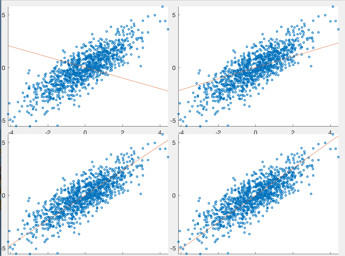
Example 1:

The figure below shows the first few iterations of the PPCA based on the EM method presented above, for a set of $N=1000$ data points in ${\bf X}=[{\bf x}_1,\cdots,{\bf x}_N]$ the $d=2$ dimensional space. The stright line in the plots indicates the direction of ${\bf w}_1$, which is initially set along a random direction, but quickly approaches the direction corresponding to the principal component obtained by the PCA method, along which the data points are most widely spread.

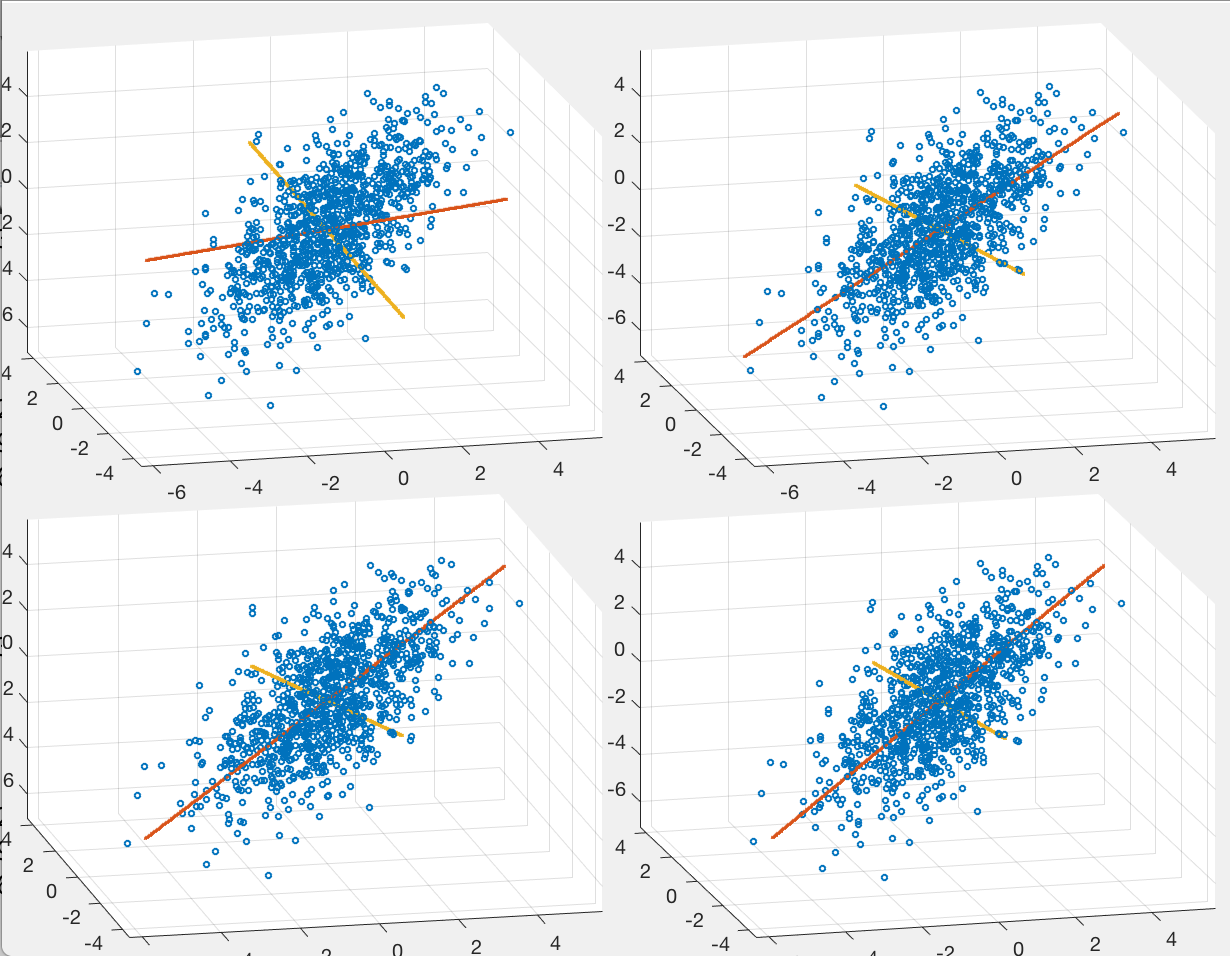
Example 2:

The figure below shows the first few iterations of the PPCA EM algorithm for a set of data points in $d=3$ dimensional space. The stright lines in the plots indicates the direction of the principal components when $d'=2$.

Example 3:

The figure below shows the visualization of the dataset for the hand-written numbers from 0 to 9, containing 2240 data points in a 256-D space, but now linearly mapped to a 3-D space spanned by $d'=3$ factors found by the PPCA method.