Next: Independent Component Analysis Up: ch8 Previous: Classical Multidimensional Scaling
It is impossible to reduce the dimensionality of a given dataset which is intrinsically high-dimensional (high-D), while still preserving all the pairwise distances in the resulting low-dimensional (low-D) space, compromise will have to be made to sacrifice certain aspects of the dataset when the dimensionality is reduced.
The PCA method as a linear, dimensionality reduction algorithm,
is unable to interpret complex nonlinear relationship between features. tance preserving method, the PCA emphasizes the importance of the PCA dimensions with great variances, but neglects small distance variations. It places distant and dissimilar data points far apart in the low-D space, while ignoring the importance of similar datapoints close together in the high-D, which need to be also placed close together in the low-D space. Therefore the PCA method tends to preserve large scale global structure of the dataset, while ignoring the small scale local structure.
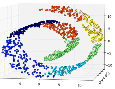
But in some cases the local structures are of equal or even more importance than the global ones, such as the typical example of “Swiss roll”.
Also, when the dimensionality is much reduced from a high-D space to a low-D space, the crowding problem occurs. In a high-D space, a data point may have a large number of similar neighbors of roughly equal distance; however, in a low-D space, the number of equal-distance neighbors is significantly reduced (8 in a 3-D space, 4 in a 2-D space, 2 in a 1-D space). Thus the space available for the neighbors of a point is much reduced. As the result, when a large number of neighbors in the high-D are mapped to a low-D space, they are forced to spread out, some are getting closer to those that are farther away in the original space, thereby reducing the gaps between potential clusters of similar points.
In contrast, the t-SNE method is a nonlinear method that is based on probability distributions of the data points being neighbors, and it attempts to preserve the structure at all scales, but emphasizing more on the small scale structures, by mapping nearby points in high-D space to nearby points in low-D space.
The similarity between any two distinct points  and
and  in the high-D space is defined as a probability based on the Gaussian kernel:
 |
(185) |
 ,
,  is defined to be zero, as it
never needed in the algorithm. Note that
is defined to be zero, as it
never needed in the algorithm. Note that  is a probability measurement
as it is normalized and add up to 1.
is a probability measurement
as it is normalized and add up to 1.
If is close to ,
 is small
and is large, indicating is similar to ;
but if is far away from ,
is large and is small, indicating is dissimilar to
. Also, as
is small
and is large, indicating is similar to ;
but if is far away from ,
is large and is small, indicating is dissimilar to
. Also, as
 , can be considered as
a probability that any two points and are neighbors
in the feature space and are therefore similar to each other.
, can be considered as
a probability that any two points and are neighbors
in the feature space and are therefore similar to each other.
Similarly, we could also define the similarity  in the low-D space
also based on the Gaussian kernel. However, for reason explained below,
we prefer to define the similarity
in the low-D space
also based on the Gaussian kernel. However, for reason explained below,
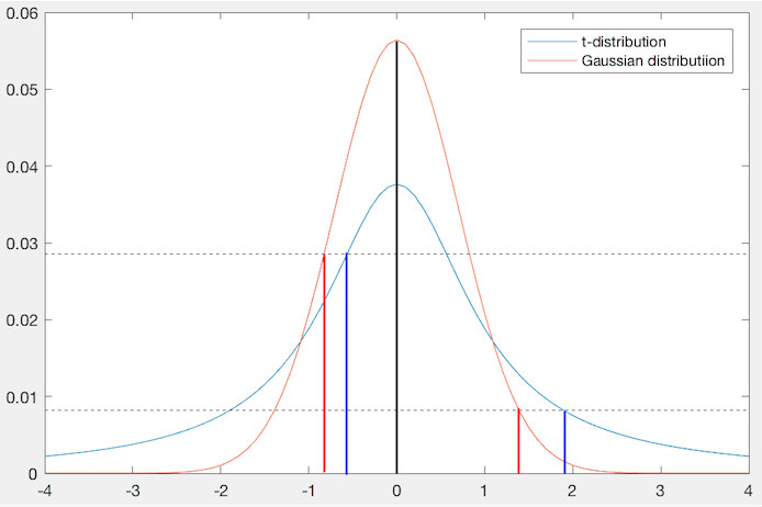
we prefer to define the similarity  in the low-D space based on
Student's t-distribution of degree 1, instead of Gaussian distribution:
in the low-D space based on
Student's t-distribution of degree 1, instead of Gaussian distribution:
 |
(186) |
be the point of interest (black, in
the center of the Gaussian kernel), then another point (red) is
mapped to a different position, which is closer to if they are
initially close (similar), or farther away from each other if they are
initially far apart (dissimilar).
How well the points  in the low-D space represent the similarity
relationship among the points in the original high-D space can
be measured by the discrepancy bwtween the two sets of probabilities,
measured by the cost function, defined as the
Kullback-Leibler divergence:
in the low-D space represent the similarity
relationship among the points in the original high-D space can
be measured by the discrepancy bwtween the two sets of probabilities,
measured by the cost function, defined as the
Kullback-Leibler divergence:
 |
(187) |
in the low-D space
that minimize the discrepancy
 .
.
The KL divergence is not symmetric as
 ,
therefore it can not be viewed as a distance between the two sets of
probabilities. This asymmetry is actually a desired feature. Consider
the following two cases:
,
therefore it can not be viewed as a distance between the two sets of
probabilities. This asymmetry is actually a desired feature. Consider
the following two cases:
is large but is small, the cost  is very large,
i.e., and such a mapping is heavily penalized. As the result, similar
points that are close to each other in the high-D space tend to be mapped
to points in the low-D space that are also close to each other.
is very large,
i.e., and such a mapping is heavily penalized. As the result, similar
points that are close to each other in the high-D space tend to be mapped
to points in the low-D space that are also close to each other.
is small but is large, the cost is small,
i.e., such a mapping is not heavily penalized. As the result, dissimilar
points that are far apart in the high-D space are allowed to be mapped to
points in the low-D space that are closer to each other.
Before proceeding to consider the minimization of the cost function ,
we still need to resolve two additional issues:
defined above is that when a point
is an outlier with large distances
to every other point in the dataset, is small and
insignificant in the cost function , and the location of
in the low-D space can not be well determined. To resolve this issue, we
redefine as the average of two conditioinal probablities:
 |
(188) |
 is the total number of data points and
 |
(189) |
is a neighboring
point similar to a given point . Note that  is properly
normalized and add up to 1:
is properly
normalized and add up to 1:
 |
(190) |
 for depending on the local data density
in the neighborhood of . Specifically, we choose in such
a way that the perplexity
for depending on the local data density
in the neighborhood of . Specifically, we choose in such
a way that the perplexity
 is the same for all data points, i.e., the entropy
 representing the uncertainty is the same,
independent of the local data density. As shown
here, the entropy of a
Gaussian
representing the uncertainty is the same,
independent of the local data density. As shown
here, the entropy of a
Gaussian
 is
is
 , a monotonic function
of its variance
, a monotonic function
of its variance  .
.
We can now find the optimal map points that minimize the cost
function
, by gradient descent method.
To find the gradient of
 , we first introduce a
set of intermediate variables
, we first introduce a
set of intermediate variables
 |
(191) |
 |
(192) |
![$\displaystyle \frac{\partial Z}{\partial d_{ij}}
=\frac{\partial}{\partial d_{ij}} \left[\sum_k\sum_{l\ne k}(1+d_{kl}^2)^{-1}\right]
=-2d_{ij}(1+d_{ij}^2)^{-2}$](img716.svg) |
(193) |
based on chain-rule. Note that when
changes, only  and
and  (for all
  ) change, we therefore
have
) change, we therefore
have
 |
(194) |
![$\displaystyle \frac{\partial d_{ij}}{\partial{\bf y}_i}
=\frac{\partial d_{ji}}...
...f y}_j)\right]^{-1/2}2({\bf y}_i-{\bf y}_j)
=\frac{{\bf y}_i-{\bf y}_j}{d_{ij}}$](img720.svg) |
(195) |
 |
(196) |
 . Note that only
  may be a
function of , while all
may be a
function of , while all  are constants, we therefore have
 |
 |
![$\displaystyle \frac{\partial}{\partial d_{ij}}
\left[\sum_k\sum_{l\ne k} \left(...
...right]
=-\sum_k\sum_{l\ne k} p_{kl} \frac{\partial}{\partial d_{ij}}\log q_{kl}$](img726.svg) |
|
|
 |
||
|
 |
||
|
![$\displaystyle 2d_{ij}\left[\frac{p_{ij}}{q_{ij}} \frac{(1+d_{ij}^2)^{-2}}{Z}-\frac{(1+d_{ij}^2)^{-2}}{Z}\right]$](img729.svg) |
(197) |
 when
when  or
or  ,
and the last equality is due to
,
and the last equality is due to
 . But as
 |
(198) |
 |
(199) |
with
respect to each of the map points :
 |
|
 |
|
|
 |
(200) |
Given the gradient vector, we can iteratively approach the optimal data
points in the low-D space that minimize the discrepancy
:
 |
(201) |
 is the step size (learning rate) and the second term
is momentum term.
is the step size (learning rate) and the second term
is momentum term.