Cubic Spline Interpolation

All previously discussed methods of polynomial interpolation fit a set of $n+1$ given points $y_i=f(x_i),\;(i=0,\cdots,n)$ by an nth degree polynomial, and a higher degree polynomial is needed to fit a larger set of data points. A major drawback of such methods is overfitting, as domonstrated by the following example.

Example:

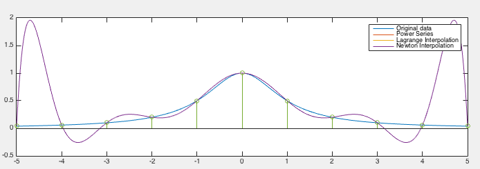
Vased on $n+1=11$ equally spaced points from $x_0=-5$ to $x_{10}=5$ with increment of 1, a function $y=f(x)=1/(1+x^2)$ can be approximated by any of the interpolation methods discussed above by polynomial of degree $n=10$, as shown in the figure below. We note that the approximation is very poor towards to the two ends where the error $R_n(x)=f(x)-N_n(x)$ is disappointingly high. This is known as Runge's phenomenon, indicating the fact that higher degree polynomial interpolation does not necessarily always produce more accurate result, as the degree of the interpolating polynomial may become unnecessarily high and the polynomial may become oscillatory.

This Runge's phenominon is a typical example of overfitting, due to an excessively complex model with too many parameters relative to the observed data, here specifically a polynomial of a degree too high (requiring too many coefficients) to model the given data points.

Now we consider a different method of spline interpolation, which fits the given points by a piecewise polynomial function $S(x)$, known as the spline, a composite function formed by $n$ low-degree polynomials $P_i(x)$ each fitting $f(x)$ in the interval between $x_{i-1}$ and $x_i,\;(i=1,\cdots,n)$:

$$S(x)=\left\{\begin{array}{cc}P_1(x) & x_0\le x\le x_1\\ \vdots &... ...e x\le x_i\\ \vdots & \vdots\\ P_n(x) & x_{n-1}\le x\le x_n\end{array}\right.$$ (61)

As this method does not use a single polynomial of degree $n$ to fit all $n+1$ points at once, it avoids high degree polynomials and thereby the potential problem of overfitting. These low-degree polynomials need to be such that the spline $S(x)$ they form is not only continuous but also smooth.

• For $S(x)$ to be continuous, two consecutive polynomials $P_i(x)$ and $P_{i+1}(x)$ must join at $x_i$:

  $$P_i(x_i)=P_{i+1}(x_i)=f(x_i)=y_i$$ (62)

  Or, equivalently, $P_i(x)$ must pass the two end-points, i.e.,

  $$P_i(x_{i-1})=f(x_{i-1})=y_{i-1},\;\;\;\;\;P_i(x_i)=f(x_i)=y_i$$ (63)

• For $S(x)$ to be smooth, they need to have the same derivatives at the point they joint, i.e.,

  $$P_i^{(k)}(x_i)=P_{i+1}^{(k)}(x_i)$$ (64)

  must hold for some order $k$. The higher the order $k$ is, the more smooth the spline $S(x)$ becomes.

In the following we consider approximating $f(x)$ between any two consecutive points $x_i$ and $x_{i+1}$ by a linear, quadratic, and cubic polynomial $P_i(x)$ (of first, second, and third degree).

• Linear spline: $P_i(x)=a_ix+b_i$ with two parameters $a_i$ and $b_i$ can only satisfy the following two equations required for $S(x)$ to be continuous:

  $$P_i(x_i)=a_ix_i+b_i=f(x_i)=y_i,\;\;\;\;\;\;\;\; P_i(x_{i-1})=a_ix_{i-1}+b_i=f(x_{i-1})=y_{i-1}$$ (65)

  or, equivalently, $P_i(x)$ has to pass the two end points $(x_{i-1},\,y_{i-1})$ and $(x_i,\,y_i)$:

  $$\frac{P_i(x)-y_{i-1}}{x-x_{i-1}}=\frac{y_i-y_{i-1}}{x_i-x_{i-1}}$$ (66)

  Solving either of two problems above, we get:
  

  $$P_i(x) = a_ix+b_i =\frac{y_i-y_{i-1}}{h_i}\,x+\frac{x_iy_{i-1}-x_{i-1}y_i}{h_i}$$

  $$= \frac{x-x_{i-1}}{h_i}y_i+\frac{x_i-x}{h_i}y_{i-1}, \;\;\;\;\;\;\;\;\;\; (h_i=x_i-x_{i-1})$$ (67)

  
  which is represented in the form of $P_i(x)=a_ix+b_i$ by the first expression, or a linear interpolation of the two end points $y_{i-1}=f(x_{i-1})$ and $y_i=f(x_i)$ in the second expression.

  As $P_i(x_i)=P_{i+1}(x_i)=y_i$, the linear spline $S(x)$ is continuous at $x_i$. But as in general

  $$P'_i(x_i)=\frac{y_i-y_{i-1}}{h_i}\ne P'_{i+1}(x_i)=\frac{y_{i+1}-y_i}{h_i}$$ (68)

  $S(x)$ is not smooth, i.e., $k=0$.

• Quadratic spline: $Q_i(x)=a_ix^2+b_ix+c_i$ with three parameters $a_i,\;b_i$ and $c_i$ can satisfy the following three equations required for $S(x)$ to be smooth ($k=1$) as well as continuous:

  $$Q_i(x_i)=y_i,\;\;\;\;Q_i(x_{i-1})=y_{i-1}, \;\;\;\;Q'_i(x_i)=Q'_{i+1}(x_i)$$ (69)

  To obtain the three parameters $a_i$, $b_i$ and $c_i$ in $Q_i(x)$, we consider $Q'_i(x)=2a_ix+b_i$, which, as a linear function, can be linearly fit by the two end points $f'(x_{i-1})=D_{i-1}$ and $f'(x_i)=D_i$:

  $$Q'_i(x)=\frac{x-x_{i-1}}{h_i}D_i+\frac{x_i-x}{h_i}D_{i-1}$$ (70)

  Integrating, we get

  $$Q_i(x)=\int Q'_i(x)\,dx=\frac{D_i}{2h_i}(x-x_{i-1})^2 -\frac{D_{i-1}}{2h_i}(x_i-x)^2+c_i$$ (71)

  As $Q_i(x_i)=y_i$, we have

  $$Q_i(x_i)=\frac{D_i}{2h_i}(x_i-x_{i-1})^2+c_i=\frac{D_ih_i}{2}+c_i=y_i$$ (72)

  Solving this for $c_i$

  $$c_i=y_i-\frac{D_ih_i}{2}$$ (73)

  and substituting it back into the expression of $Q_i(x)$, we get

  $$Q_i(x)=\frac{D_i}{2h_i}(x-x_{i-1})^2-\frac{D_{i-1}}{2h_i}(x_i-x)^2 +y_i-\frac{D_ih_i}{2}$$ (74)

  Also, as $Q_i(x_{i-1})=y_{i-1}$, we have

  $$Q_i(x_{i-1})=-\frac{D_{i-1}h_i}{2}+y_i-\frac{D_ih_i}{2}=y_{i-1}$$ (75)

  or

  $$D_i=2\frac{y_i-y_{i-1}}{h_i}-D_{i-1},\;\;\;\;\;\;(i=1,\cdots,n)$$ (76)

  Given $f'(x_0)=D_0$, we can get iteratively all subsequent $D_1,\cdots,D_n$ and thereby $Q_i(x)$. Alternatively, given $f'(x_n)=D_n$, we can also get iteratively all previous $D_{n-1},\cdots,D_0$. It is obvious that with only three free parameters, the quadratic polynomials cannot satisfy both boundary conditions $Q'_1(x_0)=f'(x_0)$ and $Q'_n(x_n)=f'(x_n)$.

• Cubic spline: $C_i(x)=a_ix^3+b_ix^2+c_ix+d_i$ with four parameters $a_i,\;b_i,\;c_i$, and $d_i$ can satisfy the following four equations required for $S(x)$ to be continuous and smooth ($k=2$):

  $$C_i(x_i)=y_i,\;\;\;\;C_i(x_{i-1})=y_{i-1},\;\;\;\; C'_i(x_i)=C'_{i+1}(x_i),\;\;\;\;\;\; \;\;\;\;\; C''_i(x_i)=C''_{i+1}(x_i)$$ (77)

  To obtain the four parameters $a_i$, $b_i$, $c_i$ and $d_i$ in $C_i(x)$, we first consdier $C''_i(x)=(a_ix^3+b_ix^2+c_ix+d_i)''=6a_ix+2b_i$, which, as a linear function, can be linearly fit by the two end points $f''(x_{i-1})=M_{i-1}$ and $f''(x_i)=M_i$:

  $$C''_i(x)=\frac{x_i-x}{h_i} M_{i-1}+\frac{x-x_{i-1}}{h_i} M_i$$ (78)

  Integrating $C''_i(x)$ twice we get

  $$C_i(x)=\int\left(\int C''_i(x)\,dx\right)\;dx =\frac{(x_i-x)^3}{6h_i}M_{i-1}+\frac{(x-x_{i-1})^3}{6h_i}M_i+c_ix+d_i$$ (79)

  As $C_i(x_{i-1})=y_{i-1}$ and $C_i(x_i)=y_i$, we have:

  $$C_i(x_{i-1})=\frac{h_i^2}{6}M_{i-1}+c_ix_{i-1}+d_i=y_{i-1}, \;\;\;\;\;\;\;\; C_i(x_i)=\frac{h_i^2}{6}M_i+c_ix_i+d_i=y_i$$ (80)

  Solving these two equations we get the two coefficients $c_i$ and $d_i$:

  $$c_i=\frac{y_i-y_{i-1}}{h_i}-\frac{h_i}{6}(M_i-M_{i-1})$$ (81)

  $$d_i=\frac{x_iy_{i-1}-x_{i-1}y_i}{h_i}-\frac{h_i}{6}(x_iM_{i-1}-x_{i-1}M_i)$$ (82)

  Substituting them back into $C_i(x)$ and rearranging the terms we get
  

  $$C_i(x) = \frac{(x_i-x)^3}{6h_i}M_{i-1}+\frac{(x-x_{i-1})^3}{6h_i}M_i +\left(\frac{y_i-y_{i-1}}{h_i}-\frac{h_i}{6}(M_i-M_{i-1})\right)x$$

  $$+\frac{x_iy_{i-1}-x_{i-1}y_i}{h_i}-\frac{h_i}{6}(x_iM_{i-1}-x_{i-1}M_i)$$

  $$= \frac{(x_i-x)^3}{6h_i}M_{i-1}+\frac{(x-x_{i-1})^3}{6h_i}M_i +\left(\frac{y_{i-1}}{h_i}-\frac{M_{i-1}h_i}{6}\right) (x_i-x)$$

  $$+\left(\frac{y_i}{h_i}-\frac{M_ih_i}{6}\right) (x-x_{i-1})$$ (83)

  
  To find $M_i$ $(i=1,\cdots,n-1)$, we take derivative of $C_i(x)$ and rearrange terms to get
  

  $$C'_i(x) = -\frac{(x_i-x)^2}{2h_i}M_{i-1}+\frac{(x-x_{i-1})^2}{2h_i}M_i -\fr... ...\frac{M_{i-1}h_i^2}{6}\right) +\frac{1}{h_i}\left(y_i-\frac{M_ih_i^2}{6}\right)$$

  $$= -\frac{(x_i-x)^2}{2h_i}M_{i-1}+\frac{(x-x_{i-1})^2}{2h_i}M_i +\frac{y_i-y_{i-1}}{h_i}-\frac{h_i}{6}(M_i-M_{i-1})$$ (84)

  
  which, when evaluated at $x=x_i$ and $x=x_{i-1}$, becomes:
  

  $$C'_i(x_i) = \frac{h_i}{3}M_i+\frac{y_i-y_{i-1}}{h_i}+\frac{h_i}{6}M_{i-1} =\frac{h_i}{6}(2M_i+M_{i-1})+f[x_{i-1},x_i]$$

  $$C'_i(x_{i-1}) = -\frac{h_i}{3}M_{i-1}+\frac{y_i-y_{i-1}}{h_i} -\frac{h_i}{6}M_i =-\frac{h_i}{6}(2M_{i-1}-M_i)+f[x_{i-1},x_i]$$ (85)

  
  Replacing $i$ by $i+1$ in the second equation, we also get

  $$C'_{i+1}(x_i)=-\frac{h_{i+1}}{3}M_i+\frac{y_{i+1}-y_i}{h_{i+1}} -\frac{h_{i+1}}{6}M_{i+1}$$ (86)

  To satisfy $C'_i(x_i)=C'_{i+1}(x_i)$, we equate the above to the first equation to get:

  $$\frac{h_i}{3}M_i+\frac{y_i-y_{i-1}}{h_i}+\frac{h_i}{6}M_{i-1} =-\frac{h_{i+1}}{3}M_i+\frac{y_{i+1}-y_i}{h_{i+1}}-\frac{h_{i+1}}{6}M_{i+1}$$ (87)

  Multiplying both sides by $6/(h_{i+1}+h_i)=6/(x_{i+1}-x_{i-1})$ and rearranging, we get:

  $$\frac{h_i}{h_{i+1}+h_i}M_{i-1}+2M_i+\frac{h_{i+1}}{h_{i+1}+h_i}M_... ...y_{i+1}-y_i}{h_{i+1}} -\frac{y_i-y_{i-1}}{h_i}\right)=6\,f[x_{i-1},x_i,x_{i+1}]$$ (88)

  Note that here

  $$\frac{1}{x_{i+1}-x_{i-1}}\left(\frac{y_{i+1}-y_i}{x_{i+1}-x_i} -\... ...ght) =\frac{f[x_i,x_{i+1}]-f[x_{i-1},x_i]}{x_i-x_{i-1}} =f[x_{i-1},x_i,x_{i+1}]$$ (89)

  is simply the second divided differences. We can rewrite the equation above as

  $$\mu_iM_{i-1}+2M_i+\lambda_iM_{i+1}=6\,f[x_{i-1},x_i,x_{i+1}],\;\;\;\;\;\;\; (i=1,\cdots,n-1)$$ (90)

  where

  $$\mu_i=\frac{h_i}{h_{i+1}+h_i},\;\;\;\; \lambda_i=\frac{h_{i+1}}{h_{i+1}+h_i}=1-\mu_i$$ (91)

  Here we have $n-1$ equations but $n+1$ unknowns $M_0,\cdots,M_n$. To obtain these unknowns, we need to get two additional equations based on certain assumed boundary conditions.
  • Assume the first order derivatives at both ends $f'(x_0)$ and $f'(x_n)$ are known. Specially $f'(x_0)=f'(x_n)=0$ is called clamped boundary condition. At the front end, we set

    $$C'_1(x_0)=-\frac{h_1}{3}M_0+\frac{y_1-y_0}{h_1}-\frac{h_1}{6}M_1 =-\frac{h_1}{3}M_0-\frac{h_1}{6}M_1+f[x_0,x_1]=f'(x_0)$$ (92)

    Multiplying $-6/h_1=-6/(x_1-x_0)$ we get

    $$2M_0+M_1=\frac{6}{x_1-x_0}[f[x_0,x_1]-f'(x_0)]=6\,f[x_0,x_0,x_1]$$ (93)

    Similarly, at the back end, we also set

    $$C'_n(x_{n})=\frac{h_n}{3}M_n+\frac{y_n-y_{n-1}}{h_n} +\frac{h_n}{6}M_{n-1} =\frac{h_n}{3}M_n+\frac{h_n}{6}M_{n-1}+f[x_{n-1},x_n]=f'(x_n)$$ (94)

    Multiplying $6/h_n=6/(x_n-x_{n-1})$ we get

    $$2M_n+M_{n-1}=\frac{6}{x_n-x_{n-1}}[f'(x_n)-f[x_{n-1},x_n]] =6\,f[x_{n-1},x_n,x_n]$$ (95)

    We can combine Eqs [?], [?] and [?] into a linear equation system of $n+1$ equations and the same number of unknowns:

    $$\left[\begin{array}{ccccc} 2 & 1 & & & \\ \mu_1 & 2 & \lambda_1 ... ...,x_2]\\ \vdots\\ f[x_{n-2},x_{n-1},x_n]\\ f[x_{n-1},x_n,x_n] \end{array}\right]$$ (96)

  • Alternatively, we can also assume $f''(x_0)$ and $f''(x_n)$ are known. Specially $f''(x_0)=f''(x_n)=0$ is called natural boundary condition. Now we can simply get $M_0=f''(x_0)$ and $M_n=f''(x_n)$ and solve the following system for the $n+1$ unknowns $M_0,\cdots,M_n$:

    $$\left[\begin{array}{ccccc} 1 & 0 & & & \\ \mu_1 & 2 & \lambda_1 ... ...f[x_0,x_1,x_2]\\ \vdots\\ 6f[x_{n-2},x_{n-1},x_n]\\ f''(x_n) \end{array}\right]$$ (97)

Example:

A function $y=f(x)=x\,\sin(2x+\pi/4)+1$ is sampled at the following $n+1=4$ points:

$$\begin{array}{c\vert\vert c\vert c\vert c\vert c}\hline i & 0... ...(x_i) & 1.937 & 1.000 & 1.349 & -0.995 \\ \hline \end{array}\\$$

The interpolation results based on linear, quadratic and cubic splines are shown in the figure below, together with the original function $f(x)$, and the $n=3$ interpolating polynomials $P_i(x), \;Q_i(x),\;C_i(x),\;(i=1,\cdots,3)$, used as the ith segment of $S(x)$ between $x_{i-1}$ and $x_i$.

For the quadratic interpolation, based on $D_0=f'(x_0)=-1.635$ we get $D_1=-0.240,\;D_2=0.937,\;D_3=-5.624$. For the cubic interpolation, we solve the following equation

$$\left[\begin{array}{llll}2 & 1 & 0 & 0\\ 0.5 & 2 & 0.5 & 0\\ 0 &... ...ht] =\left[\begin{array}{r}4.185\\ 3.858\\ -8.076\\ 9.827\end{array}\right] \\$$

and get $M_0=0.281,\;M_1=3.622,\;M_2=-7.054,\;M_3=8.440$.

The errors of these three methods are $\epsilon=0.2103$, $\epsilon=0.4371$, and $\epsilon=0.0615$, respectively. Obviously the higher the degree of the interpolating polynomial, the higher the accuracy. The error of the cubic spline method is significantly smaller than $\epsilon=0.3063$ of the polynomial interpolation.

The Matlab code that implements the cubic spline method is listed below.

function [S C]=Spline3(u,x,y,dya,dyb)
    % vectors x and y contain n+1 points and the corresponding function values
    % vector u contains all discrete samples of the continuous argument of f(x)
    % dya and dyb are the derivatives f'(x_0) and f'(x_n), respectively 
    n=length(x);       % number of interpolating points
    k=length(u);       % number of discrete sample points
    C=zeros(n,k);      % the n-1 cubic interpolating polynomials
    A=2*eye(n);        % coefficient matrix on left-hand side
    A(1,2)=1;
    A(n,n-1)=1;   
    d=zeros(n,1);      % vector on right-hand side
    d(1)=((y(2)-y(1))/(x(2)-x(1))-dya)/h0;  % first element of d
    for i=2:n-1
        h0=x(i)-x(i-1);
        h1=x(i+1)-x(i);
        h2=x(i+1)-x(i-1);       
        A(i,i-1)=h0/h2;
        A(i,i+1)=h1/h2;
        d(i)=((y(i+1)-y(i))/h1-(y(i)-y(i-1))/h0)/h2; % 2nd divided difference
    end
    d(n)=(dyb-(y(n)-y(n-1))/h1)/h1;   % last element of d
    M=6*inv(A)*d;                     % solving linear equation system for M's
    for i=2:n
        h=x(i)-x(i-1);
        x0=u-x(i-1);
        x1=x(i)-u;
        C(i-1,:)=(x1.^3*M(i-1)+x0.^3*M(i))/6/h... % the ith cubic polynomial
                 -(M(i-1)*x1+M(i)*x0)*h/6+(y(i-1)*x1+y(i)*x0)/h;  
        idx=find(u>x(i-1) & u<=x(i));  % indices between x(i-1) and x(i)
        S(idx)=C(i-1,idx);             % constructing spline by cubic polynomials
    end
end

Example:

The function $y=f(x)=1/(1+x^2)$ used before is now approximated by both the Newton's method and the cubic spline method, with very different results as shown below. The Runge's phenomenon suffered by Newton's method is certainly avoided by the cubic spline method.