Hermite Interpolation

If the first $m$ derivatives of the function $f(x)$ are known as well as the function value at each of the $n+1$ node points $x_0,\cdots,x_n$, i.e., we have available a set of $(n+1)(m+1)$ values $y_j^{(i)}=f^{(i)}(x_j), ;(j=0,\cdots,n,\;i=0,\cdots,m)$, then the function can be interpolated by a polynomial of degree $(n+1)(m+1)-1$:

$$H_{(n+1)(m+1)-1}(x)=\sum_{k=0}^{(n+1)(m+1)-1} c_kx^k$$ (46)

In principle, the $(n+1)(m+1)$ coefficients $c_0,\,c_1, \cdots,c_{(n+1)(m+1)-1}$ could be obtained by solving a linear equation system of the same number of equations:

$$\frac{d^i}{dx^i}H(x)\bigg\vert _{x=x_j} =\frac{d^i}{dx^i}\left(\s... ...right)\bigg\vert _{x=x_j} =f^{(i)}(x_j),\;\;\;\;\;(j=0,\cdots,n,\;i=0,\cdots,m)$$ (47)

As the solution of this equation system, the coefficients are unique. However, this method is impractical due to its high computational complexity $O((mn)^3)$.

In practice, the Hermite interpolation can be used in such a case. First, we assume $m=1$, and represent the Hermite polynomial as a linear combination of $(n+1)(m+1)=2(n+1)$ basis polynomials $\alpha_i(x),\;\beta_i(x)$ ( $i=0,\cdots,n$) of degree $2n+1$:

$$H(x)=\sum_{i=0}^n \alpha_i(x)\;f(x_i)+\sum_{i=0}^n \beta_i(x)\;f'(x_i)$$ (48)

In order for $H(x)$ to satisfy $H(x_j)=f(x_j)$ and $H'(x_j)=f'(x_j)$ ( $j=0,\dots,n$), the basis polynomials must satisfy:

$$\alpha_i(x_j)=\beta'_i(x_j)=\delta_{ij},\;\;\;\; \alpha'_i(x_j)=\beta_i(x_j)=0,\;\;\;\;\;\;(i,j=0,\cdots,n)$$ (49)

Since the nth degree Lagrange polynomial $l_i(x)$ satisfies $l_i(x_j)=\delta_{ij}$, we let the basis polynomials of degree $2n+1$ take the following forms:

$$\alpha_i(x)=(ax+b)\;l_i^2(x),\;\;\;\;\;\;\beta_i(x)=(cx+d)\;l_i^2(x), \;\;\;\;\;(i=0,\cdots,n)$$ (50)

Now we need to determine the four parameters $a,\,b,\,c$ and $d$ for $\alpha_i(x)$ and $\beta_i(x)$ to satisfy the following when $x=x_i$:

$$\begin{array}{l} \left\{\begin{array}{l} \alpha_i(x_i)=(ax_i+... ...^2(x_i)+(cx_i+d)\;2l'_i(x_i)=c=1 \end{array}\right. \end{array}$$ (51)

Solving these two pairs of equations we get

$$\left\{\begin{array}{l} a=-2l'_i(x_i)\\ b=1+2x_i l'_i(x_i) \end{array}\right. \;\;\;\;\;\;\; \;\;\;\;\;\;\; \left\{\begin{array}{l} c=1\\ d=-x_i \end{array}\right.$$ (52)

and

$$\left\{\begin{array}{l} \alpha_i(x)=(ax+b)l_i^2(x)=(1-2l'_i(x)(x-x_i))\;l_i^2(x)\\ \beta_i(x)=(cx+d)l_i^2(x)=(x-x_i)\;l_i^2(x) \end{array}\right.$$ (53)

Now the Hermite interpolation polynomial can be found to be:

$$H(x) = \sum_{i=0}^n \alpha_i(x)\;f(x_i)+\sum_{i=0}^2\beta_i(x)\;f'(x_i)$$

$$= \sum_{i=0}^n (1-2l'_i(x)(x-x_i))\; l_i^2(x)\;f(x_i) +\sum_{i=0}^n (x-x_i)\;l_i^2(x)\;f'(x_i)$$

$$= \sum_{i=0}^n\left[f(x_i)+(x-x_i)(f'(x_i)-2f(x_i)l'_i(x))\right]\;l_i^2(x)$$ (54)

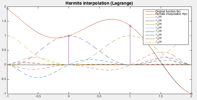
Example

The Hermite interpolation is carried out to the same function $y=f(x)=x\,\sin(2x+\pi/4)+1$ used in previous examples, with the result shown in the figure below, together with the basis polynomials $\alpha_i(x), \beta_i(x),\;(i=0,\cdots,3)$. As the first order derivative $f'(x_i)$ is available as well as the function value $f(x_i)$ at each node point $x_i$, the interpolation $H(x)$ matches the given function $f(x)$ very well (almost identical on the plots), with an error $\epsilon=0.0040$, which is much reduced from $\epsilon=0.3063$ of all methods previously discussed based only on $f(x_i)$.

The Matlab code that implements the Hermite interpolation method is listed below.

function [H a b]=HIL(u,x,y,dy)  % Hermite interpolation (Lagrange)
                         % u: discrete data points; 
                         % vector x: [x_1,...,x_n]
                         % vector y: [y_1,...,y_n]
                         % vector dy: [y'_1,...,y'_n]
   n=length(x);          % number of interpolating points
   k=length(u);          % number of discrete data points
   li=ones(n,k);         % Lagrange basis polynomials
   a=zeros(n,k);         % basis polynomials alpha(x)
   b=zeros(n,k);         % basis polynomials beta(x)    
   H=zeros(1,k);         % Hermie interpolation polynomial H(x)
   for i=1:n       
       dl=0;             % derivative of Lagrange basis
       for j=1:n    
           if j~=i
               dl=dl+1/(x(i)-x(j));
               li(i,:)=li(i,:).*(u-x(j))/(x(i)-x(j)); 
           end
       end
       l2=li(i,:).^2;
       b(i,:)=(u-x(i)).*l2;           % basis polynomial alpha(x)
       a(i,:)=(1-2*(u-x(i))*dl).*l2;  % basis polynomial beta(x)
       H=H+a(i,:)*y(i)+b(i,:)*dy(i);  % Hermite polynomial H(x)
   end   
end

We next consider the case when $m>1$. Now we have $m+1$ known values $f(x_i),\,f'(x_i),\cdots,f^{(m)}(x_i)$ at each of the node points $x_0,\cdots,x_n$. Such a dataset can be represented by another variable $z$ that takes the values of $x_0,\cdots,x_n$ each repeated $m$ times, as shown in the table:

$$\begin{array}{c\vert c\vert c\vert c\vert\vert c\vert\vert c\... ...& f(x_n) & f'(x_n) &\cdots & f^{(m)}(x_n) \\ \hline \end{array}$$ (55)

This function $f(z)$ with $(n+1)(m+1)$ sample points can then be interpolated by the Newton polynomial method. For example, if $m=n=2$, then the Newton's polynomial of degree $(2+1)(2+1)-1=8$ can be found to be:

$$N_8(x) = f(z_0)+\sum_{i=1}^8 f[x_0,\cdots,x_i]\prod_{j=0}^{i-1}(x-x_j)$$

$$= f(z_0)+f[z_0,z_1](x-z_0)+f[z_0,z_1,z_2](x-z_0)(x-z_1)$$

$$+f[z_0,\cdots,z_3](x-z_0)(x-z_1)(x-z_2)$$

$$+f[z_0,\cdots,z_4](x-z_0)(x-z_1)(x-z_2)(x-z_3)$$

$$+f[z_0,\cdots,z_5](x-z_0)(x-z_1)(x-z_2)(x-z_3)(x-z_4)$$

$$+f[z_0,\cdots,z_6](x-z_0)(x-z_1)(x-z_2)(x-z_3)(x-z_4)(x-z_5)$$

$$+f[z_0,\cdots,z_7](x-z_0)(x-z_1)(x-z_2)(x-z_3)(x-z_4)(x-z_5)(x-z_6)$$

$$+f[z_0,\cdots,z_8](x-z_0)(x-z_1)(x-z_2)(x-z_3)(x-z_4)(x-z_5)(x-z_6)(x-z_7)$$

$$= f(x_0)+f[x_0,x_0](x-x_0)+f[x_0,x_0,x_0](x-x_0)^2+f[x_0,x_0,x_0,x_1](x-x_0)^3$$

$$+f[x_0,x_0,x_0,x_1,x_1](x-x_0)^3(x-x_1)+f[x_0,x_0,x_0,x_1,x_1,x_1](x-x_0)^3(x-x_1)^2$$

$$+f[x_0,x_0,x_0,x_1,x_1,x_1,x_2](x-x_0)^3(x-x_1)^3$$

$$+f[x_0,x_0,x_0,x_1,x_1,x_1,x_2,x_2](x-x_0)^3(x-x_1)^3(x-x_2)$$

$$+f[x_0,x_0,x_0,x_1,x_1,x_1,x_2,x_2,x_2](x-x_0)^3(x-x_1)^3(x-x_2)^2$$ (56)

It can be verified that indeed $N_8^{(i)}(x_j)=f^{(i)}(x_j)$ for all $i=0,\cdots,m$ and $j=0,\cdots,n$. Similar to the Newton polynomial method discussed previously, the divided difference coefficients can be obtained recursively, with the only difference that there exist $m+1$ repeated copies at each point $x_i$, where the divided difference can be found by

$$f[x_0,\cdots,x_0]=\lim\limits_{x_i\rightarrow x_0,\;(i=0,\cdots,n)} f[x_0,\cdots,x_n] =\frac{f^{(n)}(x_0)}{n!}$$ (57)

The divided difference coefficients in the expression of $N_8(x)$ above can be recursively generated in tabular form below, eventually appearing as the diagonal elements of the table.

$$\begin{array}{c\vert c\vert\vert c\vert c\vert c\vert c\vert ... ...f[x_1,x_2,x_2,x_2] &f[x_1,x_1,x_2,x_2,x_2]\\ \hline \end{array}$$ (58)

$$\begin{array}{c\vert c\vert c\vert c}\hline 5th & 6th & 7th &... ..._2]&f[x_0,x_0,x_0,x_1,x_1,x_1,x_2,x_2,x_2]\\ \hline \end{array}$$ (59)

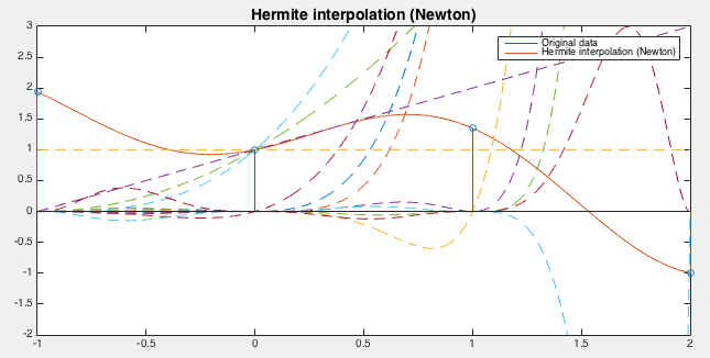
Example:

The Hermite interpolation based Newton's polynomials is again carried out to the same function $y=f(x)=x\,\sin(2x+\pi/4)+1$ used before. Now we assume both the first and second order derivatives $f'(x_i)$ and $f''(x_i)$ are available as well as $f(x_i)$ at the $n+1=4$ points. The resulting Hermite interpolation $H(x)$ is plotted together with $f(x)$ in the figure below. We see that they are almost identical, with an error $\epsilon=6.5\times 10^{-6}$.

The Matlab code that implements this algorithm is listed below.

function [v]=HIN(u,x,dy)         % Hermite interpolation (Newton)
    % u: discrete data points; 
    % vector x: [x_1,...,x_n]
    % matrix dy contains m derivatives at each of the n points 
    [n m]=size(dy);              
    k=length(u);                 % number of discrete data points
    v=zeros(1,k);                % interpolation results    
    dd=DividedDifference2(x,dy); % get the divided difference array
    w=ones(1,k);  
    for i=1:n
        p=u-x(i);
        for j=1:m
            l=(i-1)*m+j;         % index of the coefficient 
            v=v+dd(l,l).*w;      % which is on the diagnal of array dd
            w=w.*p;
        end
    end    
end

function dd=DividedDifference2(x,dy)  % generate array of divided differences
    [n m]=size(dy);              % n data points, m derivatives (0 to m-1)
    dd=zeros(n*m);               % matrix of divided differences
    z=zeros(1,n*m); 
    k=1;
    for i=1:n                    % n data points
        for j=1:m                % m derivatives (0 to m-1) at each point
            k=(i-1)*m+j;         % row index
            z(k)=x(i);      
            dd(k,1)=dy(i,1);     % 0th divided difference in first column
            fprintf('%6.3f\t%6.3f\t',z(k),dd(k,1));
            for l=2:k            % column index for the remaining columns
                %fprintf('(%f %f)\n',dd(k,l-1),dd(k-1,l-1));
                if dd(k,l-1)==dd(k-1,l-1)  % left and top-left neighbors are repeated
                    dd(k,l)=dy(i,l)/factorial(l-1);
                    fprintf('k=%d, l=%d\n',k,l);
                    pause
                else                       
                    dd(k,l)=(dd(k,l-1)-dd(k-1,l-1))/(z(k)-z(k-l+1));
                end
                fprintf('%6.3f\t',dd(k,l));
            end
            fprintf('\n');
        end
    end
end

The array of divided differences generated by the function DividedDifference2 is given below, the elements along the diagonal are the coefficients in the Hermite polynomials.

$$\begin{array}{r\vert\vert r\vert r\vert r\vert r\vert r\vert ... ...0.0172 & 0.0220 & 0.0028 &-0.0007 &-0.0002\\ \hline \end{array}$$ (60)