The Newton Polynomial Interpolation

The Lagrange interpolation relies on the $n+1$ interpolation points $\{x_i,\,y_i=f(x_i),\;i=0,\cdots,n\}$, all of which need to be available to calculate each of the basis polynomials $l_i(x)$. If additional points are to be used when they become available, all basis polynomials need to be recalculated.

In comparison, in the Newton interpolation, when more data points are to be used, additional basis polynomials and the corresponding coefficients can be calculated, while all existing basis polynomials and their coefficients remain unchanged. Due to the additional terms, the degree of interpolation polynomial is higher and the approximation error may be reduced (e.g., when interpolating higher order polynomials).

Specifically, the basis polynomials of the Newton interpolation are calculated as below:

$$n_0(x)=1,\;\;\;\;n_i(x)=\prod_{j=0}^{i-1}(x-x_j),\;\;\;\;\;\;(i=1,\cdots,n)$$ (25)

and the Newton interpolating polynomial is constructed:

$$N_n(x) = \sum_{i=0}^n c_i n_i(x)=c_0+\sum_{i=1}^n c_i\; \left(\prod_{j=0}^{i-1}(x-x_j)\right)$$

$$= c_0+c_1(x-x_0)+c_2(x-x_0)(x-x_1)+\cdots+c_n\prod_{j=0}^{n-1}(x-x_j)$$ (26)

When when the next data point $(x_n, y_n)$ is available, not used in any of the basis polynomials, but it is used for calculating the last coefficient $c_n$, as shown below. For this nth degree polynomial $N_n(x)$ to pass all $n+1$ points $(x_i,\;y_i),\;(i=0,\cdots,n)$, it needs to satisfy the following $n+1$ equations:

$$\left\{\begin{array}{l} y_0=c_0\\ y_1=c_0+c_1(x_1-x_0)\\ y_2=c_... ...)+c_2(x_n-x_0)(x_n-x_1)+\cdots+c_n\prod_{i=0}^{n-1}(x_n-x_i) \end{array}\right.$$ (27)

which can also be expressed in matrix form:

$$\left[\begin{array}{cccccc}1&&&&&\\ 1&x_1-x_0&&&&\\ 1&x_2-x_0&(x... ...] =\left[\begin{array}{c}y_0\\ y_1\\ y_2\\ y_3\\ \vdots\\ y_n\end{array}\right]$$ (28)

The $n+1$ coefficients $c_0,\cdots,c_n$ can be obtained by solving these $n+1$ equations in the triangular equation system progressively from top down:

$$c_0 = y_0=f(x_0)=f[x_0]$$

$$c_1 = \frac{y_1-y_0}{x_1-x_0}=f[x_0,x_1]$$

$$c_2 = \frac{\frac{y_2-y_0}{x_2-x_0}-\frac{y_1-y_0}{x_1-x_0}}{x_2-x_1} =f[x_0,x_1,x_2]$$

$$= \frac{y_0}{(x_0-x_2)(x_0-x_1)}+\frac{y_1}{(x_1-x_0)(x_1-x_2)} +\frac{y_2}{(x_2-x_0)(x_2-x_1)}$$

$$c_3 = \frac{\frac{\frac{y_3-y_0}{x_3-x_0}-\frac{y_1-y_0}{x_1-x_0}}{x_3-... ..._2-y_0}{x_2-x_0}-\frac{y_1-y_0}{x_1-x_0}}{x_2-x_1}}{x_3-x_2} =f[x_0,\cdots,x_3]$$

$$= \frac{y_0}{(x_0-x_1)(x_0-x_2)(x_0-x_3)} +\frac{y_1}{(x_1-x_0)(x_1-x_2)(x_1-x_3)}$$

$$+\frac{y_2}{(x_2-x_0)(x_2-x_1)(x_2-x_3)} +\frac{y_3}{(x_3-x_0)(x_3-x_1)(x_3-x_2)}$$

$$\cdots \cdots\cdots\cdots\cdots$$ (29)

In general, we have

$$c_k=f[x_0,\cdots,x_k] =\sum_{j=0}^k\frac{f(x_j)}{\prod_{i=0,\;i\ne j}^k (x_j-x_i)}, \;\;\;\;\;(k=0,\cdots,n)$$ (30)

which is the expanded form of the kth divided differences $f[x_0,\cdots,x_k]$ of the first $k+1$ points. Now the Newton polynomial interpolation can be written as

$$N_n(x)=\sum_{i=0}^nc_i n_i(x)=\sum_{i=0}^n f[x_0,\cdots,x_i] n_i(x) =f[x_0]+\sum_{i=1}^n\;f[x_0,\cdots,x_i]\left(\prod_{j=0}^{i-1}(x-x_j)\right)$$ (31)

Due to the uniqueness of the polynomial interpolation, this Newton interpolation polynomial is the same as that of the Lagrange and the power function interpolations: $N_n(x)=L_n(x)=P_n(x)$. They are the same nth degree polynomial but expressed in terms of different basis polynomials weighted by different coefficients.

We can now consider some important facts all related to the Newton polynomial interpolation.

• When an additional node point $(x_{n+1},\,y_{n+1})$ is avialable and to be used, all previous basis polynomials and their corresponding coefficients remain unchanged, we only need to obtain a new basis polynomial of degree $n+1$:

  $$n_{n+1}(x)=n_n(x)(x-x_n)=\prod_{i=0}^{n-1}(x-x_i)(x-x_n) =\prod_{i=0}^n(x-x_i)=l(x)$$ (32)

  together with its coefficient, the (n+1)th divided difference $c_{n+1}=f[x_0,\cdots,x_n,x_{n+1}]$. The new interpolation polynomial of degree $n+1$ can then be obtained by including an extra term in the summation above:

  $$N_{n+1}(x)=\sum_{i=0}^{n+1}c_i n_i(x) =\sum_{i=0}^n c_i n_i(x)+c_{n+1}n_{n+1}(x) =N_n(x)+f[x_0,\cdots,x_n,x_{n+1}] l(x)$$ (33)

  As $N_{n+1}(x)$ passes through the new point $(x_{n+1},\,y_{n+1})$, we have

  $$f(x_{n+1})=N_{n+1}(x_{n+1})=N_n(x_{n+1})+f[x_0,\cdots,x_n,x_{n+1}] l(x)$$ (34)

  But $x_{n+1}$ is just an arbitrary point, we can replace it by $x$, and get

  $$f(x)=N_n(x)+f[x_0,\cdots,x_n,x] l(x)$$ (35)

  Comparing this with the error function:

  $$R_n(x)=f(x)-N_n(x)=\frac{f^{(n+1)}(\xi)}{(n+1)!} l(x)$$ (36)

  we see that the error term can also be written as

  $$R_n(x)=f[x_0,\cdots,x_n,\,x] l(x)$$ (37)

  and we also get:

  $$f[x_0,\cdots,x_n,x]=\frac{f^{(n+1)}(\xi)}{(n+1)!}$$ (38)

• Specially, if all of the $n+1$ node points approach to a single position, $x_i\rightarrow x_0,\;(i=1,\cdots,n)$, at the limit they become the same point $x_0$ repeated $n$ times, then we have

  $$f[x_0,\cdots,x_n]=\frac{f^{(n)}(\xi)}{n!} \;\;\;\stackrel{x_i\rightarrow x_0}{\Longrightarrow}\;\;\; f[x_0,\cdots,x_0]=\frac{f^{(n)}(x_0)}{n!}$$ (39)

  and the Newton interpolation based on $n+1$ points becomes

  $$N_n(x)=f[x_0]+\sum_{i=1}^n \left(f[x_0,\cdots,x_i]\prod_{j=0}^{i-... ...rrow x_0}{\Longrightarrow} f(x_0)+\sum_{i=1}^n \frac{f^{(i)}(x_0)}{i!}(x-x_0)^i$$ (40)

  which is the first $n+1$ terms of the Taylor series expansion of the function with the truncation error:

  $$R_n(x)=\frac{f^{(n+1)}(\xi)}{(n+1)!}\prod_{i=0}^n(x-x_i) \stackrel{x_i\rightarrow x_0}{\Longrightarrow} \frac{f^{(n+1)}(\xi)}{(n+1)!}(x-x_0)^{n+1}$$ (41)

  where $\xi$ is some point between $x$ and $x_0$. We see that the Taylor series is actually a special case of the Newton interpolation at the limit when all $n+1$ node points approach to the same position $x_0$.

• If all $n+1$ points $x_0=a\le x_1\le\cdots\le x_{n-1}\le x_n=b$ are equally spaced, i.e.,

  $$x_{i+1}-x_i=h=\frac{b-a}{n},\;\;\;\;\;(i=0,\cdots,n-1)$$ (42)

  then Newton's divided difference interpolation can take a simpler form. For any point $x\in(a,\,b)$, we let $c=(x-x_0)/h$ so that it can be represented as $x=x_0+ch$, and $x-x_i=(x_0+ch)-(x_0+ih)=(c-i)h$, now the Newton polynomial can be written as
  

  $$N(x) = N(x_0+ch)=f[x_0]+\sum_{i=1}^nf[x_0,\cdots,x_i]\prod_{j=0}^{i-1}(x-x_j)$$

  $$= f[x_0]+f[x_0,x_1]ch+f[x_0,x_1,x_2]c(c-1)h^2 +\cdots+f[x_0,\cdots,x_n]c(c-1)\cdots(c-n+1)h^n$$

  $$= \sum_{i=0}^nf[x_0,\cdots,x_i]c(c-1)(c-2)\cdots(c-i+1)h^i =\sum_{i=0}^nf[x_0,\cdots,x_i]\left(\begin{array}{c}c\\ i\end{array}\right)i!\;h^i$$ (43)

  
  where

  $$\left(\begin{array}{c}c\\ i\end{array}\right) =\frac{c!}{i!(c-i)!} =\frac{c(c-1)(c-2)\cdots(c-i+1)}{i!}$$ (44)

Example: Approximate function $y=f(x)=x\,\sin(2x+\pi/4)+1$ by a polynomial of degree $n=3$, based on the following $n+1=4$ points:

$$\begin{array}{c\vert\vert c\vert c\vert c\vert c}\hline i & 0... ...(x_i) & 1.937 & 1.000 & 1.349 & -0.995 \\ \hline \end{array}\\$$

Based on $f[x_i]=f(x_i),\;(i=0,\cdots,n)$, we can find all other divided differences recursively in tabular form as shown below. In general, $f[x_i,\cdots,x_j]$ can be found based on its left neighbor $f[x_{i+1},\cdots,x_j]$ and top-left neighbor $f[x_i,\cdots,x_{j-1}]$:

$$f[x_i,\cdots,x_j]=\frac{f[x_{i+1},\cdots,x_j]-f[x_i,\cdots,x_{j-1}]}{x_j-x_i} \\$$

$$\begin{array}{c\vert\vert l\vert l\vert l\vert l}\hline x_i &... ... f[x_1,x_3]=-1.346 & f[x_0,x_3]=-0.663 \\ \hline \end{array}\\$$

The coefficients are the four divided differences along the diagonal: $c_0=f[x_0]=f(x_0)=y_0=1.937$, $c_1=f[x_0,x_1]=-0.937$, $c_2=f[x_0,x_1,x_2]=0.643$, and $c_3=f[x_0,x_1,x_2,x_3]=-0.663$. Alternatively, they can also be represented in the expanded form:

$$c_i=f[x_0,\cdots,x_i]=\sum_{j=0}^n\frac{f(x_j)}{\prod_{i=0,\,i\ne j}^n(x_j-x_i)}$$ (45)

Now the Newton interpolating polynomial can be obtained as:

$$N_3(x) = \sum_{i=0}^3 c_i n_i(x)$$

$$= 1.937-0.937(x+1)+0.643(x+1)(x-0)-0.663(x+1)(x-0)(x-1)$$

$$= 1+0.369\,x+0.643\,x^2-0.663\,x^3$$

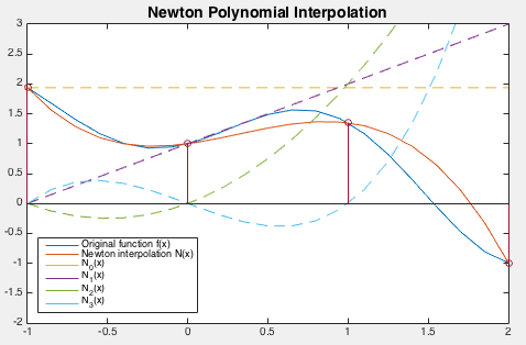
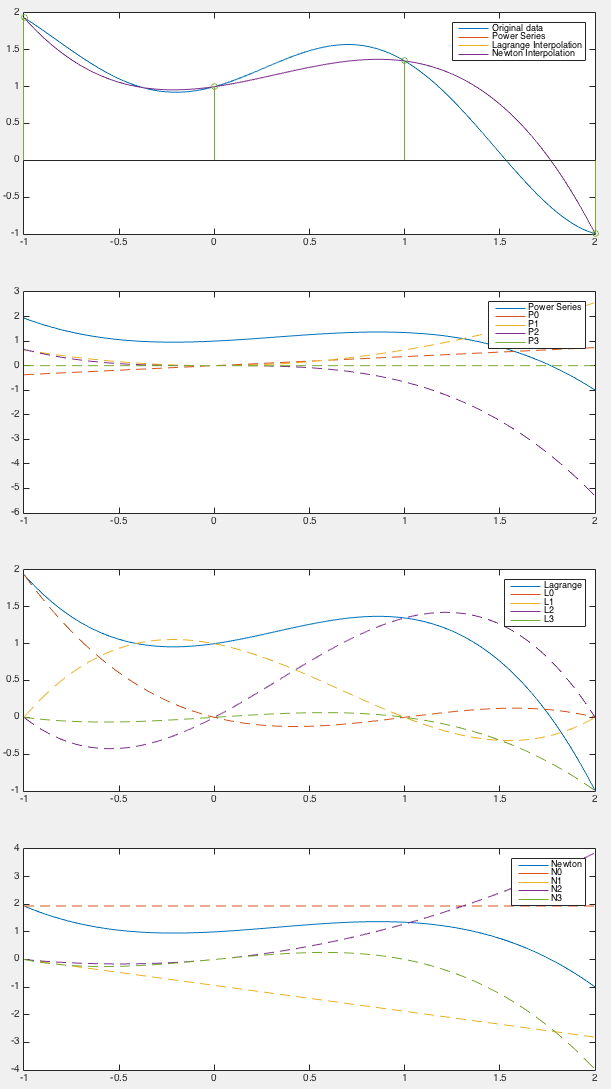
The polynomial interpolations generated by the power series method, the Lagrange and Newton interpolations are exactly the same, $P_3(x)=L_3(x)=N_3(x)$, confirming the uniqueness of the polynomial interpolation, as plotted in the top panel below, together with the original function $y=f(x)$. We see that they indeed pass through all $n+1=4$ node points at $x_0=-1$, $x_1=0$, $x_2=1$ and $x_3=2$. Also, the weighted basis polynomials of each of the three methods are plotted in the subsequent panels, including power series $a_0x^0,\cdots,a_3x^3$ in the second panel, the Lagrange basis polynomials $y_0l_0(x),\cdots,y_3l_3(x)$ in the third panel, and the Newton basis polynomials $c_0n_0(x),\cdots, c_3n_3(x)$ in the bottom panel. In each case, the weighted sum of these basis polynomials is the interpolating polynomial that approximates the given function.

The Matlab code that implements the Newton polynomial method is listed below. The coefficients $c_i=f[x_0,\cdots,x_n]\;(i=0,\cdots,n)$ can be generated in either the expanded form or the tabular form by recursion.

function [v N]=NI(u,x,y)  % Newton's Interpolation
    % vectors x and y contain n+1 points and the corresponding function values
    % vector u contains all discrete samples of the continuous argument of f(x)
    n=length(x);          % number of interpolating points
    k=length(u);          % number of discrete sample points
    v=zeros(1,k);         % Newton interpolation 
    N=ones(n,k);          % all n Newton's polynomials (each of m elements)
    N(1,:)=y(1);          % first Newton's polynomial
    v=v+N(1,:);    
    for i=2:n             % generate remaining Newton's polynomials
        for j=1:i-1
            N(i,:)=N(i,:).*(u-x(j));   
        end
        c=DividedDifference(x,y,i)  % get the ith coefficient c_i
        v=v+c*N(i,:);     % weighted sum of all Newton's polynomials
    end
end

function dd=DividedDifference(x,y,i) % generate f[x_0,...,x_i] in expanded form
    dd=0;
    for k=1:i             % loop for summation
        de=1;
        for l=1:i         % loop for product
            if k~=l   
                de=de*(x(k)-x(l));               
            end
        end
        dd=dd+y(k)/de;    % ith coefficient c_i
    end
end

function dd=DividedDifferenceMatrix(x,y) % generate divided difference matrix
    n=length(x);                         % the coefficients are along diagonal
    dd=zeros(n);                         % matrix of divided differences
    dd(:,1)=y;
    for i=1:n
        fprintf('%6.3f\t',dd(i,1))
        for j=2:i
            dd(i,j)=(dd(i,j-1)-dd(i-1,j-1))/(x(i)-x(i-j+1));
            fprintf('%6.3f\t',dd(i,j));
        end
        fprintf('\n');
    end
end