Polynomial Interpolation

It is often needed to estimate the value of a function $y=f(x)$ at certan point $x$ based on the known values of the function $f(x_0), \cdots,f(x_n)$ at a set of $n+1$ node points $a=x_0\le x_1\le\cdots\le x_n=b$ in the interval $[a,\; b]$. This process is called interpolation if $a<x<b$ or extrapolation if either $x<a$ or $b<x$. One way to carry out these operations is to approximate the function $f(x)$ by an nth degree polynomial:

$$f(x)\approx P_n(x)=a_nx^n+a_{n-1}x^{n-1}+\cdots+a_2x^2+a_1x+a_0 =\sum_{j=0}^n a_jx^j$$ (1)

where the $n+1$ coefficients $a_0,\cdots,a_n$ can be obtained based on the $n+1$ given points. Once $P_n(x)$ is available, any operation applied to $f(x)$, such as differentiation, intergration, and root finding, can be carried out approximately based on $P_n(x)\approx f(x)$. This is particulary useful if $f(x)$ is non-elementary and therefore difficult to manipulate, or it is only available as a set of discrete samples without a closed-form expression.

Specifically, to find the coefficients of $P_n(x)$, we require it to pass through all node points $\{x_i,y_i=f(x_i),\;i=0,\cdots,n\}$, i.e., the following $n+1$ linear equations hold:

$$P_n(x_i)=\sum_{j=0}^n a_jx^j_i=f(x_i)=y_i,\;\;\;\;(i=0,\cdots,n)$$ (2)

Now the coefficients $a_0,\cdots,a_n$ can be found by solving these $n+1$ linear equations, which can be expressed in matrix form as:

$$\left[ \begin{array}{ccccc} 1 & x_0 & x_0^2 & \cdots & x_0^n \\ ... ...\left[\begin{array}{c}y_0\\ y_1\\ y_2\\ \vdots\\ y_n\end{array}\right] ={\bf y}$$ (3)

where ${\bf a}=[a_0,\cdots,a_n]^T$, ${\bf y}=[y_0,\cdots,y_n]^T$, and

$${\bf V}=\left[ \begin{array}{ccccc} 1 & x_0 & x_0^2 & \cdots & x_... ...vdots & \ddots & \vdots \\ 1 & x_n & x_n^2 & \cdots & x_n^n \end{array}\right]$$ (4)

is known as the Vandermonde matrix. Solving this linear equation system, we get the coefficients $[a_0,\cdots,a_n]^T={\bf a}={\bf V}^{-1}{\bf y}$. Here $n+1$ polynomials $x^0, x^1, x^2,\cdots,x^n$ can be considered as a set of polynomial basis functions that span the space of all nth degree polynomials (which can also be spanned by any other possible bases). If the node points $x_0,\cdots,x_n$ are distinct, i.e., ${\bf V}$ has a full rank and its inverse ${\bf V}^{-1}$ exists, then the solution of the system ${\bf a}={\bf V}^{-1}{\bf f}$ is unique and so is $P_n(x)$.

In practice, however, this method is not widely used for two reasons: (1) the high computational complexity $O(n^3)$ for calculating ${\bf V}^{-1}$, and (2) matrix ${\bf V}$ becomes more ill-conditioned as $n$ increases. Instead, other methods to be discussed in the following section are practically used.

The error of the polynomial interpolation is defined as

$$R_n(x)=f(x)-P_n(x)$$ (5)

which is non-zero in general, except if $x=x_i$ at which $R_n(x_i)=0,\;(i=0,\cdots,n)$. In other words, the error function $R_n(x)$ has $n+1$ zeros at $x_0,\cdots,x_n$, and can therefore be written as

$$R_n(x)=u(x)\prod_{i=0}^n(x-x_i)=u(x) l(x)$$ (6)

where $u(x)$ is an unknown function and $l(x)$ is a polynomial of degree $n+1$ defined as

$$l(x)=\prod_{i=0}^n(x-x_i)$$ (7)

To find $u(x)$, we construct another function $F(t)$ of variable $t$ with any $x\in(a,\,b)$ as a parameter:

$$F(t)=R_n(t)-u(x)\prod_{i=0}^n(t-x_i)=f(t)-P_n(t)-u(x)\prod_{i=0}^n(t-x_i)$$ (8)

which is zero when $t=x$:

$$F(x)=R_n(x)-u(x)\prod_{i=0}^n(x-x_i)=R_n(x)-R_n(x)=0$$ (9)

We therefore see that $F(t)$ has $n+2$ zeros at $x_0,\cdots,x_n$ and $x$. According to Rolle's theorem, which states that the derivative function $f'(x)$ of any differentiable function $f(x)$ satisfying $f(a)=f(b)=0$ must have at least a zero at some point $c\in(a,\;b)$ at which $f'(c)=0$, $F'(t)$ has at least $n+1$ zeros each between two consecutive zeros of $F(t)$, $F''(t)$ has at least $n$ zeros, and $F^{(n+1)}(t)$ has at least one zero at some $\xi\in(a,\;b)$:

$$F^{(n+1)}(\xi)=0 = \frac{d^{n+1}}{dt^{n+1}} \left[ f(t)-P_n(t)-u(x)\prod_{i=0}^n(t-x_i) \right]_{t=\xi}$$

$$= \left[f^{(n+1)}(t)+P_n^{(n+1)}(t)-u(x)\frac{d^{n+1}}{dt^{n+1}}\prod_{i=0}^n(t-x_i)\right]_{t=\xi}$$

$$= f^{(n+1)}(\xi)-u(x)(n+1)!$$ (10)

The last equation is due to the fact that $P_n(t)$ and $\prod_{i=0}^n(t-x_i)$ are respectively an nth and (n+1)th degree polynomials of $t$. Solving the above we get

$$u(x)=\frac{f^{(n+1)}(\xi)}{(n+1)!}$$ (11)

Now the error function can be written as

$$R_n(x)=u(x)\prod_{i=0}^n(x-x_i)=\frac{f^{(n+1)}(\xi)}{(n+1)!}\,l(x)$$ (12)

where $\xi(x)$ is a point located anywhere between $a=x_0$ and $b=x_n$ dependending on $x$. The error can be quantitatively measured by the 2-normal of $R_n(x)$:

$$\epsilon=\vert\vert R_n(x)\vert\vert _2=\left(\int_a^b R^2_n(x)\,dx\right)^{1/2}$$ (13)

In particular, if $f(x)$ is a polynomial of degree $k\le n$, then $f^{(n+1)}(x)=0$, and it can be exactly interpolated by $P_n(x)$. But if $k>n$, the interpolation has a non-zero error term $R_n(x)$. In particular, if $f(x)$ is a polynomial of degree $n+1$, such as $f(x)=x^{n+1}$, then $f^{(n+1)}(x)=(n+1)!$ and the error term becomes:

$$R_n(x)=\frac{f^{(n+1)}(\xi)}{(n+1)!}\,l(x)=l(x)$$ (14)

Due to the uniqueness of the polynomial interpolation, the error analysis above also applies to all other methods to be considered in the following sections, such as the Lagrange and Newton interpolations.

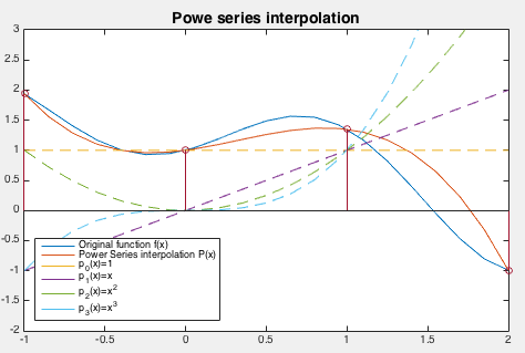
Example:

Approximate function $y=f(x)=x\,\sin(2x+\pi/4)+1$ by a polynomial $P_3(x)$ of degree $n=3$, based on the following $n+1=4$ node points:

$$\begin{tabular}{c\vert\vert c\vert c\vert c\vert c}\hline i & 0 &... ...\hline $y_if(x_i)$\ & 1.937 & 1.000 & 1.349 & -0.995 \\ \hline \end{tabular}\\$$

We first find the Vandermonde matrix:

$${\bf V}=\left[ \begin{array}{cccc} 1 & x_0 & x_0^2 & x_0^3 \\ 1 ... ...-1 \\ 1 & 0 & 0 & 0 \\ 1 & 1 & 1 & 1 \\ 1 & 2 & 4 & 9 \end{array}\right] \\$$

and get the coefficients:

$${\bf a}={\bf V}^{-1}{\bf y}={\bf V}^{-1} \left[\begin{array}{r}f(... ...ht] =\left[\begin{array}{r}1.000\\ 0.369\\ 0.643\\ -0.663\end{array}\right] \\$$

and then the interpolating polynomial can be found as a weighted sum of the first $n+1=4$ power functions used as the basis functions to span the polynomial space:

$$P_3(x)=\sum_{j=0}^na_j x^j=1.0+0.369\;x+0.643 \;x^2-0.663\;x^3 \\$$

This interpolation polynomial $P_3(x)$ is plotted in the figure below, in comparison to the orginal function $f(x)$, together with the basis polynomials, the power functions $x^i,\;(i=0,\cdots,3)$. The error $\epsilon$ can be approximated by a set of $k>>n$ discrete samples $u_1,\cdots,u_k$ of the function $f(x)$ and the interpolating polynomial $P_3(x)$:

$$\epsilon=\vert\vert R_3(x)\vert\vert _2=\left(\int_a^b R^2_3(x)\,... ...prox \left(\frac{1}{k}\sum_{i=1}^k [f(u_i)-P_3(u_i)]^2 \right)^{1/2}=0.3063 \\$$

The Matlab code that implements this method is listed below.

function [v P]=PI(u,x,y)  
    % vectors x and y contain n+1 points and the corresponding function values
    % vector u contains all discrete samples of the continuous argument of f(x)
    n=length(x);     % number of interpolating points
    k=length(u);     % number of discrete sample points
    v=zeros(1,k);    % polynomial interpolation 
    P=zeros(n,k);    % power function basis polynomials
    V=zeros(n);      % Vandermonde matrix
    for i=1:n
        for j=1:n
            V(i,j)=x(i)^(j-1);
        end
    end
    c=inv(V)*y;      % coefficients
    for i=1:n
        P(i,:)=u.^(i-1);
        v=v+c(i)*P(i,:);
    end
end