Regression as Optimization Problems

The goal of regression analysis is to model the relatiionship between a dependent variable $y$, typically a scalor, and a set of independent variables or predictors $\{x_1,\cdots,x_d\}$, represented as a column vector ${\bf x}=[x_1,\cdots,x_d]^T$ in a d-dimensional space. Here both $y$ and the components in ${\bf x}$ take numerical values.

Regression can be considered as a supervised learning method that learns the essential relationship between the dependent and independent variables, based on the training dataset containing $N$ observed data samples

$${\cal D}=\{ ({\bf x}_n,\,y_n),\; (n=1,\cdots, N) \}$$ (99)

where each ${\bf x}_n$ is labeld by $y_n$, the ground truth value corresponding to ${\bf x}$. We also represent the training set as ${\cal D}=\{{\bf X},\;{\bf y}\}$ in terms of a $d\times N$ matrix ${\bf X}=[{\bf x}_1,\cdots,{\bf x}_N]$ containing the $N$ sample points and an N-dimensional vector ${\bf y}=[y_1,\cdots,y_N]^T$ for their labelings.

More specifically, a regression algorithm is to model the relationship between independent variable ${\bf x}$ and the dependent variable $y$ by a hypothesized regression function $\hat{y}=f({\bf x},{\bf\theta})$, containing a set of parameters symbolically denoted by ${\bf\theta}=[\theta_1,\cdots,\theta_M]^T$. Geometrically this regression function $f({\bf x})$ represents curve if $d=1$, a surface if $d=2$ or a hypersurface if $d>2$.

Typically, the form of the function $f({\bf x},{\bf\theta})$ (e.g., linear, polynomial, or exponential) is determined is assumed to be known based on prior knowledge, while the parameter ${\bf\theta}$ is to be estimated by the regression algorithm, so that the predicted value $\hat{y}$ is to match the ground truth $y$ optimally is some sense, but not affected by the inevitable observation noise in the data. In other words, a regression algorithm should neither overfit nor underfit the data.

Regression analysis can also be interpreted as system modeling/identification, when the independent variable ${\bf x}$ and the dependent variable $y$ are treated respectively as the input (stimuli) and output (responses) of a system, the behavior of which is described by the relationship between such input and output modeled by the regression function $y=f({\bf x})$.

Regression analysis is also closely related to pattern recognition/classification, when the independent vector variable ${\bf x}$ in the data is treated as a set of features that characterize a pattern or opject of interest, and the corresponding dependent variable $y$ is treated as a categorical label indicating to which of a set of $K$ classes $\{C_1,\cdots,C_K\}$ a pattern ${\bf x}_n$ belongs. In this case, the modeling process of the relationship between ${\bf x}$ and $y$ becomes supervised pattern classification or recognition, to be discussed in a later chapter.

In general the regression problem can be addressed based on different philosophical viewpoints. In the frequentist point of view, the unknown model parameters in ${\bf\theta}$ are fixed deterministic variables that can be estimated based on the observed data, and a typical method based on this viewpoint is the least squares method.

Alternatively, in the Bayesian inferenceoint of view, the model parameters in ${\bf\theta}$ are random variables. Their prior probability distribution $p({\bf\theta})$ before any data are observed can be estimated based on some prior knowledge. If no such prior knowledge is available, $p({\bf w})$ can be simply a uniform distribution, i.e., all possible values of ${\bf w}$ are equally likely. Once the training set ${\bf X}$ becomes available, we can further get the posterior probability based on Bayes' theorem:

$$p({\bf\theta}\vert{\bf X}) =\frac{ p({\bf X}\vert{\bf\theta}) p({\bf\theta})} {p({\bf X})}\propto p({\bf X}\vert{\bf w}) p({\bf\theta})$$ (100)

In general, the posterior is a narrower distribution than the prior, and therefore a more accurate description of the model parameters. The output $\hat{y}=f({\bf x},{\bf\theta})$ of such a regression model based Bayesian inference is no longer a deterministic value, but a random variable described by its mean and variance.

Based on either of these two viewpoints, different regression algorithms can be used to find the parameters ${\bf\theta}$ for the model function $\hat{y}=f({\bf x},{\bf\theta})$ to fit the observed dataset ${\cal D}=\{ {\bf X},{\bf y}\}$ in some optimal way based on different criteria, as shown below.

• Least squares (LS) method:

  This frequentist method measures how well the regression function models the training data by the residual defined as $r({\bf\theta})=y-\hat{y}({\bf\theta})$, defined as the difference between the model prediction $\hat{y}({\bf\theta})=f({\bf x},{\bf\theta})$ and the ground truth labeling value $y$ corresponding to ${\bf x}$, for each of the $N$ data points in the observed data:

  $${\bf r}({\bf\theta}) =\left[\begin{array}{c}r_1\\ \vdots\\ r_N\en... ...\ \vdots\\ y_N-f({\bf x}_N,{\bf\theta})\end{array}\right] ={\bf y}-\hat{\bf y}$$ (101)

  Ideally, the residual should be zero, ${\bf r}({\bf\theta})={\bf0}$, and we can find the $M$ model parameters by solving this equation system of $N$ equations of $M$ unknowns in ${\bf\theta}$. However, as in general $N\gg M$, this system is overconstrained without a solution. We therefore can only use least squares method to find the optimal solution that minimizes the sum of squared error (SSE):

  $$\varepsilon({\theta})=\frac{1}{2}\vert\vert{\bf r}\vert\vert^2 =\... ...} \sum_{n=1}^N r_n^2 =\frac{1}{2} \sum_{n=1}^N (y_n-f({\bf x}_n,{\bf\theta}))^2$$ (102)

  Here the coefficent $1/2$ is included for mathematical convenience. When divide by the total number of samples $N$, this SSE becomes the average of all $N$ squared errors, and the error becomes the mean squared error (MSE).

• Maximum likelihood estimate (MLE):

  This Bayesian inference method measures how well the regression function models the training data $L({\bf\theta}\vert{\cal D})$ in terms of the likelihood

  of the model parameter ${\bf\theta}$ based on the observed dataset ${\cal D}=\{ {\bf X},{\bf y}\}$, which is proportional to the conditional probability of ${\cal D}$ given ${\bf\theta}$:

  $$L({\bf\theta}\vert{\cal D})\propto p({\cal D}\vert{\bf\theta}) =p({\bf y}\vert{\bf X},{\bf\theta})$$ (103)

  As we only need maximize the likelihood, the proportionality is not a concern. The optimal model parameters in ${\bf\theta}$ can be found as those that maximize the likelihood function, or equivalently the log likelihood function, for computational convenience:

  $$l({\bf\theta}\vert{\cal D})=\log L({\bf\theta}\vert{\cal D}) =\log p({\bf y}\vert{\bf X},{\bf\theta})$$ (104)

  Typically the residual $r=y-f({\bf x},{\bf\theta})$ is assumed to be zero-mean random variable with a normal probability density function (pdf):
  

  $$p(r) = p(y-f({\bf x},\,{\bf\theta}))={\cal N}(r,0,\sigma^2) =\frac{1}{\s... ...2\pi\sigma^2}} \exp\left(-\frac{(y-f({\bf x},{\bf\theta}))^2}{2\sigma^2}\right)$$

  $$= {\cal N}(y,f({\bf x},{\bf\theta}),\sigma^2)=p(y\vert{\bf x},{\bf\theta})$$ (105)

  
  The justification for this assumed normal pdf is that it has the greatest entropy or maximum uncertainty among all possible pdfs with the same variance, i.e., based on $\sigma^2$ only, such an assumption of normal pdf imposes least amount of constraint and thereby minimum bias.

  The zero-mean pdf of $r=y-f({\bf x},{\bf\theta})$ can also be considered as the pdf of $y$ with mean $f({\bf x},{\bf\theta})$, the conditional pdf $p(y\vert{\bf x},{\bf\theta})$ of $y$ given ${\bf\theta}$ as well as ${\bf x}$, based on the assumption that $y$ and ${\bf x}$ are indeed related by $y=f({\bf x},{\bf\theta})$. Then we can find the likelihood of the model parameter ${\bf\theta}$ given the $N$ samples in in the training set, all assumed to be independent and identically distributed (i.i.d.):
  

  $$L(\theta\vert{\cal D}) = p({\bf y}\vert{\bf X},\theta) =\prod_{n=1}^N p(y=y_n\vert{\bf x}_n,\theta)$$

  $$= \prod_{n=1}^N \frac{1}{\sqrt{2\pi\sigma^2}} \exp\left(-\frac{(y_n-f({\bf x}_n,{\bf\theta}))^2}{2\sigma^2}\right)$$ (106)

  
  or, equivalently, minimize the negative log likelihood function:
  

  $$-l({\bf\theta}\vert{\cal D}) = -\log L({\bf\theta}\vert{\bf X},{\bf y}) =-\log\left[\prod_{n=1}^... ...}}\exp \left(-\frac{(y_n-f({\bf x}_n,{\bf\theta}) )^2}{2\sigma^2}\right)\right]$$

  $$= -\sum_{n=1}^N \log\left[\frac{1}{\sqrt{2\pi\sigma^2}}\exp \left(-\frac{(y_n-f({\bf x},{\bf\theta}))^2}{2\sigma^2}\right)\right]$$

  $$= \frac{N}{2}\log (2\pi\sigma^2)+\frac{1}{2\sigma^2}\sum_{n=1}^N \vert\vert{\bf r}\vert\vert^2$$ (107)

  
  The first term and the coefficient $1/\sigma^2$ in the second term are both independent of $\theta$ and can therefore be dropped. We note that this result is equivalent to that in Eq. (#_#>107), i.e., we can find the optimal ${\bf\theta}$ by either maximizing the likelihood $L({\bf\theta}\vert{\cal D})$, or equivalently minimizing the sum of squares error $\varepsilon({\bf\theta})$.

• Maximum A Posteriori (MAP)

  This is also a Bayesian inference method that measures how well the regression function models the training data by the posterior probability of the parameter ${\bf\theta}$ given in Eq. (100), proportional to the product of the likelihood $L({\bf\theta}\vert{\cal D})\propto p({\cal D}\vert{\bf\theta})$ and the prior $p({\bf\theta})$. If no prior knowledge about ${\bf\theta}$ is available, then $p({\bf\theta})$ is a uniform distribution, then MAP is equivalent to MLE. However, if certain prior knowledge regarding ${\bf\theta}$ does exist, and the prior is not uniform, then the posterior better characterizes ${\bf\theta}$ than the likelihood and MAP may produce better result than MLE.

We see that regression analysis can be treated as an optimization problem, in which either the sum of squares error is minimized or the likelihood function is maximized. Also, the optimization problem is in general over-determined, as there are typically many more observed data points in the training data than the number of unknown parameters. Algorithms based on these different methods are to be considered in detail in later sections in this chapter.

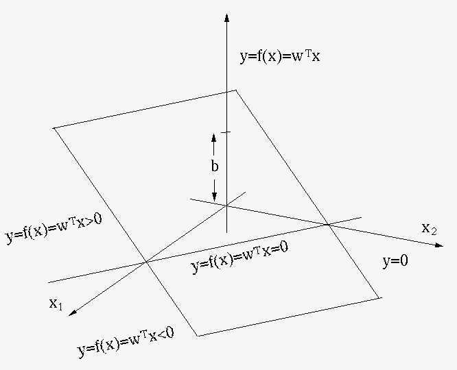
We further note that regression analysis can be considered as a binary classification, when the regression function $y=f({\bf x})$, as a hypersurface in a $d+1$ dimensional space spanned by $\{x_1,\cdots,x_d,\,y\}$, is thresholded by a constant $C$ (e.g., $C=0$). The resulting equation $f({\bf x})=C$ defines a hypersurface in the $d$ dimensional space spanned by $\{x_1,\cdots,x_d\}$, which partitions the space into two parts in such a way that all points on one side of the hypersurface satisfy $f({\bf x})>C$, while all points on the other side satisfy $f({\bf x})<C$. In other words, the regression function is a binary classifier that separates every point ${\bf x}$ in the $d$ dimensional space into two classes $C_+$ and $C_-$, depending on whether $f({\bf x})$ is greater or smaller than C. Now each $y_n$ corresponding to ${\bf x}_n$ in the given dataset ${\cal D}=\{ {\bf X},{\bf y}\}$ can be treated as a label indicating ${\bf x}_n$ belong to class $C_+$ if $y_n>C$, or $C_-$ if $y_n<C$, and the regression problem becomes a binary classification problem.