The Runge-Kutta methods

Compared with all previous discussed methods for solving a first order DE $y'(t)=f(t,y(t))$, the Runge-Kutta (RK) methods can achieve higher accuracies, i.e., the order of error term for is higher than all previous discussed methods, due to the much improved approximation of the slope of the secant $y'(t+ch)=(y(t+h)-y(t))/h,\; (0<c<1)$ between the two end points $y(t)$ and $y(t+h)$.

The general iteration of the RK methods takes the following form:

$$y(t+h)=y(t)+\Delta y_t=y(t)+h y'(t+ch) \approx y(t)+h \sum_{i=1}^s b_i k_i$$ (226)

where the slope of the secant $y'(t+ch)$ is approximated as the average of $s$ estimations $k_1,\cdots,k_s$ of the slope weighted respectively by $b_1,\cdots,b_s$:

$$y'(t+ch)\approx \sum_{i=1}^s b_i k_i$$ (227)

These $s$ estimated slopes are obtained recursively, i.e., the ith estimate $k_i$ is based on all previous estimates $k_1,\cdots,k_{i-1}$:

$$k_i=f\left(t+c_ih,\;y+h\;\sum_{j=1}^{i-1} a_{ij} k_j \right), \;\;\;\;\;\;(i=1,\cdots,s)$$ (228)

where $0\le c_i\le 1,\;c_1=0$, $b_1=1$ and $k_1=f(t+c_1 h,\,y)=f(t,\,y)$ is the slope of the tangent at $y(t)$.

This iteration can be expressed in terms of $t_n=t$, $t_{n+1}=t_n+h$, $y_n=y(t_n)$, and $f(t_n,y_n)=f_n$:

$$y_{n+1}=y_n+h \sum_{i=1}^s b_i k_i$$ (229)

where

$$k_1 = f(t_n,\;y_n)=f_n$$

$$k_2 = f\left(t_n+c_2h,\;y_n+h (a_{21}k_1)\right)$$

$$k_3 = f\left(t_n+c_3h,\;y_n+h (a_{31}k_1+a_{32}k_2)\right)$$

$$\cdots\cdots\cdots\cdots$$

$$k_s = f\left(t_n+c_s h,\;y_n+h \left(\sum_{j=1}^{s-1} a_{sj}k_j\right)\right)$$ (230)

Specially when $s=1$, we have the forward Euler method:

$$y_{n+1}=y_n+h b_1 k_1=y_n+h f_n$$ (231)

The problem of iteratively solving the DE $y'(t)=f(t,y(t))$ can also be viewed as an integral problem which can be solved by certain quadrature rules:

$$y(t+h)=y(t)+\int_t^{t+h} y'(t)\,dt =y(t)+\int_t^{t+h} f(t)\,dt\approx y(t)+\sum_{i=1}^s A_i f(t_i)$$ (232)

where $f(t_i)$ is the estimated function value $f(t)$ at some point inside the interval $[t,\,t+h]$, and $A_i$ is the corresponding weight.

In general, an s-stage RK method with free parameters $c_2,\cdots,c_s$, $b_1\cdots,b_s$ and $a_{ij},\; (i=1,\cdots,s,\;j=1,\cdots,i-1)$ can be arranged in the form of a Butcher tableau:

$$\begin{tabular}{c\vert ccccc} $c_1=0$\ &&&&& \\ $c_2$\ & $a_{21}... ...line $1$\ & $b_1$\ & $b_2$\ & $\cdots$\ & $b_{s-1}$\ & $b_s$\ \\ \end{tabular}$$ (233)

The total number of parameters is $(s^2-s)/2+s+(s-1)=(s^2+3s-2)/2$.

We need to find the specific values for these parameters so that the error term of an s-stage RK method can achieve the highest possible order in terms of the step size $h$. This is done by matching the coefficients of different orders of the $h$ terms in the RK iteration with those of the corresponding Taylor expansion of the function:

$$y(t+h)=y(t)+hy'(t)+\frac{h^2}{2}y''(t)+\frac{h^3}{3!}y'''(t) +\frac{h^4}{4!}y^{(4)}(t)+O(h^5)$$ (234)

where the derivatives of $y(t)$ can be found as:

$$y'(t) = \frac{dy}{dt}=f(t,y(t))=f$$

$$y''(t) = \frac{d^2y}{dt^2}=\frac{d}{dt}f(t,y) =\frac{\partial f}{\partial t} +\frac{\partial f}{\partial y}\frac{dy}{dt} =f_t+f_yf$$

$$y'''(t) = \frac{d^3y}{dt^3}=\frac{d}{dt}(f_t+f_yf) =\frac{d}{dt}f_t+\frac{d}{dt}(f_yf) =\frac{d}{dt}f_t+f\frac{df_y}{dt}+f_y\frac{df}{dt}$$

$$= (f_{tt}+f_{ty}f) +f(f_{ty}+f_{yy}f)+f_y(f_t+f_yf) =f_{tt}+2f_{ty}f +f_{yy}f^2+f_yf_t+f_y^2f$$

$$y^{(4)} = \frac{d^4y}{dt^4} =\frac{d}{dt}(f_{tt}+2f_{ty}f+f_{yy}f^2+f_yf_t+f_y^2f)$$

$$= (f_{ttt}+f_{tty}f) +(2f_{tty}f+2f_{tyy}f^2+2f_{ty}f_t+2f_{ty}f_yf)$$

$$+ (f_{tyy}f^2+f_{yyy}f^3+2f_{yy}f_tf+2f_{yy}f_yf^2) +(f_{ty}f_t+f_{yy}f_tf+f_yf_{tt}+f_yf_{ty}f)$$

$$+ (2f_yf_{ty}f+2f_yf_{yy}f^2+f_y^2f_t+f_y^3f)$$

$$= y(t)+h f+\frac{h^2}{2!}(f_t+f_yf) +\frac{h^3}{3!}(f_{tt}+2f_{ty}f... ...h^3}{3!}f_y(f_t+f_yf) +\frac{h^4}{4!}(f_{ttt}+3f_{tty}f+3f_{tyy}f^2+f_{yyy}f^3)$$

$$+\frac{h^4}{24}f_y(f_{tt}+2f_{ty}f+f_{yy}f^2)+\frac{h^4}{8}(f_t+f_yf)(f_{ty}+f_{yy}f) +\frac{h^4}{24}(f_t+f_yf)f_y^2+O(h^5)$$ (235)

where

$$f_t=\frac{\partial f}{\partial t},\;\; f_y=\frac{\partial f}{\par... ...tial t\partial y},\;\;\; f_{yy}=\frac{\partial^2 f}{\partial y^2},\cdots \cdots$$ (236)

Substituting these into the Taylor expansion of $y(t+h)$ in Eq. (234), we get different approximations of the function with truncation errors of progressively higher orders:

$$y(t+h) = y(t)+hf+O(h^2)$$ (237)

$$= y(t)+h f+\frac{h^2}{2!}(f_t+f_yf)+O(h^3)$$ (238)

$$= y(t)+h f+\frac{h^2}{2!}(f_t+f_yf) +\frac{h^3}{3!}(f_{tt}+2f_{ty}f +f_{yy}f^2+f_yf_t+f_y^2f)+O(h^4)$$ (239)

$$= y(t)+h f+\frac{h^2}{2!}(f_t+f_yf) +\frac{h^3}{3!}(f_{tt}+2f_{ty}f... ...yy}f^2+f_yf_t+f_y^2f) +\frac{h^4}{4!}(f_{ttt}+3f_{tty}f+3f_{tyy}f^2+f_{yyy}f^3)$$

$$+\frac{h^4}{24}f_y(f_{tt}+2f_{ty}f+f_{yy}f^2)+\frac{h^4}{8}(f_t+f_yf)(f_{ty}+f_{yy}f) +\frac{h^4}{24}(f_t+f_yf)f_y^2+O(h^5)$$ (240)

$$\cdots\cdots\cdots\cdots$$

These Taylor expansions are then compared with the iterations $y(t+h)=y(t)+h \sum_{i=1}^s b_i k_i$ of RK methods of different number of stages $(s=1,\cdots,4)$ to determine the parameters required to achieve the highest possible order for the error term.

• $s=1$:

  $$y(t+h)=y(t)+h b_1k_1=y(t)+h k_1=y(t)+h\,f(t,\,f)$$ (241)

  Comparing this with the Taylor expansion in Eq. (238), we see that if $b_1=1$. This RK1 is simply Euler's forward method in Eq. (189) with a 2nd order error.

• $s=2$:

  Given $k_1=f$, we express $k_2$ as the Taylor expansion of the 2-variable function $f(t,y(t))$:

  $$k_2=f(t+c_2h,\,y+ha_{21}k_1)=f(t,\,y)+h(c_2f_t+a_{21}f_yf)+O(h^2)$$ (242)

  and the iterative step of the RK2 method becomes
  

  $$y(t+h) = y(t)+h(b_1 k_1+b_2 k_2)$$

  $$= y(t)+hb_1f+hb_2(f+hc_2f_t+ha_{21}f_yf+O(h^2))$$

  $$= y(t)+hf(b_1+b_2)+b_2h^2(c_2f_t+a_{21}f_yf)+O(h^3)$$ (243)

  
  For the RK2 method to have the third (highest possible) order error, its coefficients have to match those of the Taylor expansion in Eq. (239), and we get the following three necessary and sufficient conditions for the parameters:

  $$b_1+b_2=1,\;\;\;\;a_{21}=c_2,\;\;\;\;b_2c_2=b_2a_{21}=\frac{1}{2}$$ (244)

  There exist multiple solutions for this equation system of three equations but four unknowns. By introducing a free variable $a_{21}=x$, the remaining three variables can be determined as shown in the Butcher's tableau of the RK2:

  $$\begin{tabular}{l\vert lll} $c_1=0$\ && \\ $c_2=x$\ & $a_{21}=x$\ & \\ \hline & $b_1=1-1/2x$\ & $b_2=1/2x$\ \\ \end{tabular}$$ (245)

  Listed below are three of such solutions corresponding to $x=1,\;1/2,\;2/3$:
  • $x=c_2=a_{21}=1,\;b_1=b_2=1/2$, we have
    

    $$k_1 = f_n$$

    $$k_2 = f(t_n+h,\;y_n+hk_1)$$

    $$y_{n+1} = y_n+h(k_1+k_2)/2$$ (246)

    
    This is the trapezoidal Euler (Heun's) method in Eq. (199), which can also be obtained by the trapezoidal rule of Newton-Cotes quadrature applied to approximate the integral in the iteration:

    $$y(t_{n+1})=y(t_n)+\int_{t_n}^{t_{n+1}} f(t)\,dt \approx y(t_n)+\frac{h}{2}[f(t_n)+f(t_n+h)]$$ (247)

  • $x=c_2=a_{21}=1/2,\;b_1=0,\;b_2=1$, we have
    

    $$k_1 = f_n$$

    $$k_2 = f(t_n+h/2,\;y_n+hk_1/2)$$

    $$y_{n+1} = y_n+h k_2$$ (248)

    
    This is the midpoint method in Eq. (218).

  • $x=c_2=a_{21}=2/3,\;b_1=1/4,\;b_2=3/4$, we have
    

    $$k_1 = f_n$$

    $$k_2 = f(t_n+2h/3,\;y_n+2k_1/3)$$

    $$y_{n+1} = y_n+h(k_1+3k_2)/4$$ (249)

    
    This is called Ralston's method.

• $s=3$

  Given $k_1=f$, we express $k_2$ and $k_3$ by their corresponding Taylor expansions:
  

  $$k_2 = f(t+c_2h,\,y+ha_{21}k_1)=f(t+c_2h,\,y+ha_{21}f)$$

  $$= f+h(c_2f_t+a_{21}ff_y)+O(h^2)$$

  $$= f+h(c_2f_t+a_{21}ff_y)+\frac{h^2}{2}(c_2^2f_{tt}+2c_2a_{21}ff_{ty} +a_{21}^2f^2f_{yy})+O(h^3)$$

  $$k_3 = f(t+c_3h,\,y+h(a_{31}k_1+a_{32}k_2))$$

  $$= f+h[c_3f_t+(a_{31}f+a_{32}(f+h(c_2f_t+a_{21}ff_y)))f_y]+O(h^2)$$

  $$= f+h[c_3f_t+(a_{31}f+a_{32}(f+h(c_2f_t+a_{21}ff_y)))f_y]$$

  $$+\frac{h^2}{2}[c_3^2f_{tt}+2c_3(a_{31}f+a_{32}f)f_{ty}+(a_{31}f+a_{32}f)^2f_{yy}] +O(h^3)$$ (250)

  
  Here all terms of $h$ of order higher than two are collected in the error term $O(h^3)$. The iterative step for this RK3 method can now be written as:
  

  $$y(t+h) = y+h(b_1 k_1+b_2 k_2+b_3 k_3)$$

  $$= y+hb_1f+hb_2\left(f+h(c_2f_t+a_{21}f_yf) +\frac{h^2}{2}(c_2^2f_{tt}+2c_2a_{21}ff_{ty}+a_{21}^2f^2f_{yy})+O(h^3)\right)$$

  $$+hb_3\left(f+h[c_3f_t+(a_{31}f+a_{32}f+a_{32}h(c_2f_t+a_{21}f_yf)... ...2c_3(a_{31}f+a_{32}f)f_{ty} +(a_{31}f+a_{32}f)^2f_{yy}]+O(h^3)\right) \nonumber$$

  $$= y+h(b_1+b_2+b_3)f+h^2f_t(c_2b_2+c_3b_3)+h^2f_yf(b_2a_{21} +b_3(a_{31}+a_{32}))+h^3(b_3a_{32}(c_2f_t+a_{21}f_yf))f_y$$

  $$+\frac{h^3}{2}(b_2c_2^2+b_3c_3^2)f_{tt} +h^3(b_2c_2a_{21}+b_3c_3(... ..._{32}))ff_{ty} +\frac{h^3}{2}(b_2a_{21}^2+b_3(a_{31}+a_{32})^2)f^2f_{yy}+O(h^4)$$ (251)

  
  For the RK3 method to have the forth (highest possible) order error, its coefficients have to match those of the Taylor expansion expansion in Eq. (240), which can also be written as

  $$y(t+h)=y+hf+\frac{h^2}{2}(f_t+f_yf) +\frac{h^3}{3}f_{ty}f+\frac{h^3}{6}(f_{tt}+f_{yy}f^2+f_yf_t+f_y^2f)+O(h^4)$$ (252)

  we get the following necessary and sufficient conditions for the parameters:
  

  $$b_1+b_2+b_3=1,\;\;\;\;\; c_2b_2+c_3b_3=b_2a_{21}+b_3(a_{31}+a_{32})=\frac{1}{2}$$

  $$b_2c_2^2+b_3c_3^2=b_2a_{21}^2+b_3(a_{31}+a_{32})^2 =b_2c_2a_{21}+... ..._3(a_{31}+a_{32})=\frac{1}{3},\;\;\;\; b_3a_{32}c_2=b_3a_{32}a_{21}=\frac{1}{6}$$

  
  Simplifying we get the following 6 independent equations:
  

  $$b_1+b_2+b_3=1$$

  $$c_2=a_{21}$$

  $$c_3=a_{31}+a_{32}$$

  $$b_2c_2+b_3c_3=1/2$$

  $$b_2c_2^2+b_3c_3^2=1/3$$

  $$b_3a_{32}c_2=1/6$$

  
  There exist multiple solutions for this system of 6 equations but 8 variables, such as the two shown below, known as Kutta's method (left) and Heun's third order method (right):

  $$\begin{tabular}{c\vert cccc} $c_2=1/2$\ & $1/2$\ && \\ $c_3=1$\ ... ..._3=2/3$\ & $0$\ & $2/3$\ & \\ \hline & $1/4$\ & $0$\ & $3/4$\ \\ \end{tabular}$$ (253)

  The RK3 iterations corresponding to the two sets of parameters are respectively:

  $$\left\{ \begin{array}{l} k_1=f_n\\ k_2=f(t_n+h/2,\;y_n+hk_1/2)\\... ... k_3=f(t_n+2h/3,\;y_n+2hk_2/3)\\ y_{n+1}=y_n+h(k_1+3k_3)/4 \end{array}\right.$$ (254)

  We recognize that the first method is simply the Simpson's rule of Newton-Cotes quadrature for approximating the integral in the iteration:

  $$y(t_{n+1})=y(t_n)+\int_{t_n}^{t_{n+1}} f(t)\,dt \approx y(t_n)+\frac{h}{6}[f(t_n)+4f(t_n+h/2)+f(t_n+h)]$$ (255)

• $s=4$

  In a similar manner, we can derive (see the next section) the following eight necessary and sufficient conditions for the parameters of RK4 method for it to have a 5th order error term:
  

  $$b_1+b_2+b_3+b_4=1$$

  $$b_2c_2+b_3c_3+b_4c_4=1/2$$

  $$b_2c_2^2+b_3c_3^2+b_4c_4^2=1/3$$

  $$b_2c_2^3+b_3c_3^3+b_4c_4^3=1/4$$

  $$b_3a_{32}c_2+b_4a_{42}c_2+b_4a_{43}c_3=1/6$$

  $$b_3a_{32}c_3c_2+b_4a_{42}c_4c_2+b_4a_{43}c_4c_3=1/8$$

  $$b_3a_{32}c_2^2+b_4a_{42}c_2^2+b_4a_{43}c_3^2=1/12$$

  $$b_4a_{43}a_{32}c_2=1/24$$ (256)

  
  

  There exist multiple solutions for this system of eight equations of 13 variables, such as the classical RK4 and the 3/8 rule methods listed respectively on the left and right below.

  $$\begin{tabular}{c\vert cccc} $c_2=1/2$\ & $1/2$\ &&& \\ $c_3=1/2... ... $-1$\ & $1$\ & \\ \hline & $1/8$\ & $3/8$\ & $3/8$\ & $1/8$\ \\ \end{tabular}$$ (257)

  The RK4 iterations corresponding to the two sets of parameters are respectively:

  $$\left\{ \begin{array}{l} k_1=f_n\\ k_2=f(t_n+h/2,\;y+hk_1/2)\\ ... ...+h,\;y+hk_1-hk_2+hk_3)\\ y_{n+1}=y_n+h(k_1+3k_2+3k_3+k_4)/8 \end{array}\right.$$ (258)

  We recognize that the second method is simply the application of the Simpson's 3/8 rule of the Newton-Cotes quadrature for approximating the integral in the iteration:

  $$y(t_{n+1})=y(t_n)+\int_{t_n}^{t_{n+1}} f(t)\,dt \approx y(t_n)+\frac{h}{8}[f(t_n)+3f(t_n+h/3)+3f(t_n+2h/3)+f(t_n+h)]$$ (259)

From the above we see that up to $s=4$, the order of accuracy is the same as the number of stages of the RK method, e.g., for RK4, the order of its accuracy is the same as its stage $s=4$ (with a 5th order error term $O(h^5)$) . However, this is not the case for $s>4$, as shown in the table below:

$$\begin{tabular}{l\vert ccccccc}\hline Order of accuracy & 1 & 2 &... ...hline Number of stages & 1 & 2 & 3 & 4 & 6 & 7 & 9 .... \\ \hline \end{tabular}$$ (260)

The Matlab code for RK4 is shown below as a function which takes three arguments, the step size $h$, time moment $t$ and $y(t)$, and generates the approximation of the next value $y(t+h)=y(t)+h \hat{y'}(t+ch)$ with $\hat{y'}(t+ch)$ estimated by one of the several versions of the RK4 method, based on another function that calculate $y'(t)=f(t,y(t))$:

function y = RungeKutta4(h, t, y, k)
    k1 = f(t, y);
    switch k
        case 1
            k2 = f(t+h/2, y + h*k1/2);    
            k3 = f(t+h/2, y + h*k2/2);
            k4 = f(t+h, y + h*k3);
            y  = y + h*(k1 + 2*k2 + 2*k3 + k4)/6;
        case 2
            k2 = f(t+h/3, y + h*k1/3);
            k3 = f(t+2*h/3, y -h*k1/3 +h*k2);
            k4 = f(t+h, y + h*k1 -h*k2 +h*k3);
            y  = y + h*(k1 + 3*k2 + 3*k3 + k4)/8;
        case 3
            k2 = f(t+2*h/3, y + 2*h*k1/3);
            k3 = f(t+h/3, y + h*k1/12 +h*k2/4);
            k4 = f(t+h, y - 5*h*k1/4 +h*k2/4 +2*h*k3);
            y  = y + h*(k1 + 3*k2 + 3*k3 + k4)/8;
        case 4
             k2 = f(t+h/2, y + h*k1/2);
             k3 = f(t+h/2, y + h*k1/6 +h*k2/3);
             k4 = f(t+h, y -h*k2/2 +3*h*k3/2);
             y  = y + h*(k1 + k2 + 3*k3 + k4)/6;
        case 5
            k2 = f(t+h/2, y + h*k1/2);
            k3 = f(t+h/2, y - h*k1/2 +h*k2);
            k4 = f(t+h, y + h*k2/2 + h*k3/2);
            y  = y + h*(k1 + 3*k2 + k3 + k4)/6;
    end    
end

Example 1: Consider a simple equation $y'(t)=f(t,y(t))=\lambda y(t)$ with a closed form solution $y(t)=y(0)e^{\lambda t}$.

• RK1, same as forward Euler's method,

  $$y_{n+1}=(1+h\lambda)y_n$$ (261)

• RK2, we choose to use $c_2=a_{21}=1$ and $b_1=b_2=1/2$:
  

  $$k_1 = f_n=\lambda y_n$$ (262)

  $$k_2 = f(t_n+h,\;y_n+hk_1)=\lambda (y_n+hk_1)=\lambda(1+h\lambda)y_n$$ (263)

  
  Substituting these into the RK2 iteration, we get

  $$y_{n+1}=y_n+\frac{h}{2}(k_1+k_2)=y_n+\frac{h}{2}\lambda y_n +\frac{h}{2}\lambda(1+h\lambda)y_n=\left(1+h\lambda+\frac{(h\lambda)^2}{2}\right)y_n$$ (264)

• RK3, we choose to use $c_2=a_{21}=1/3$, $c_3=a_{32}=2/3$, $b_1=1/4$, $b_2=0$, and $b_3=3/4$:
  

  $$k_1 = f_n=\lambda y_n$$ (265)

  $$k_2 = f(t_n+h/3,\;y_n+hk_1/3)=\lambda(1+h\lambda/3)y_n$$ (266)

  $$k_3 = f(t_n+2h/3,\;y_n+2hk_2/3)=\lambda(1+2h\lambda(1+h\lambda/3)/3)y_n$$ (267)

  $$= \lambda(1+2h\lambda/3+2(h\lambda)^2/9)y_n$$ (268)

  
  Substituting these into the RK3 iteration, we get

  $$y_{n+1}=y_n+\frac{h}{4}(k_1+3k_3) =\left(1+h\lambda+\frac{1}{2}(h\lambda)^2+\frac{1}{6}(h\lambda)^3\right)y_n$$ (269)

• RK4, we choose to use $c_2=a_{21}=c_3=a_{22}=1/2$, $c_4=a_{43}=1$ and $b_1=b_4=1/6$, $b_2=b_3=1/3$:
  

  $$k_1 = f_n=\lambda y_n$$ (270)

  $$k_2 = f(t_n+h/2,\;y_n+hk_1/2)=\lambda(1+h\lambda/2)y_n$$ (271)

  $$k_3 = f(t_n+h/2,\;y_n+hk_2/2)=\lambda(1+h(\lambda(1+h\lambda/2))/2) y_n$$

  $$= \lambda(1+h\lambda/2+(h\lambda)^2/4) y_n$$ (272)

  $$k_4 = f(t_n+h,\;y_n+hk_3)=\lambda(1+h\lambda(1+h\lambda/2+(h\lambda)^2/4) y_n$$

  $$= \lambda(1+h\lambda+(h\lambda)^2/2+(h\lambda)^3/4)) y_n$$

  
  Substituting these into the RK4 iteration, we get

  $$y_{n+1}=y_n+\frac{h}{6}(k_1+2k_2+2k_3+k_4) =\left(1+h\lambda+\frac{1}{2}(h\lambda)^2+\frac{1}{6}(h\lambda)^3 +\frac{1}{24}(h\lambda)^4\right)y_n$$ (273)

We realize that the expressions inside the brackets of the iterations of the RK methods are simply the first few terms of the Taylor expansion of $e^{h\lambda}$, i.e., the iterations above are the approximations of the closed form solution $y(t+h)=y(t) e^{h\lambda}$ with truncation errors of different orders.

The RK4 method considered above is in scalar form, however, it can be easily generalized to the following vector form:

$${\bf k}_1 = {\bf f}(t_n,\,{\bf y}_n)$$

$${\bf k}_2 = {\bf f}(t_n+h/2,\,{\bf y}_n+h\,{\bf k}_1/2)$$

$${\bf k}_3 = {\bf f}(t_n+h/2,\,{\bf y}_n+h\,{\bf k}_2/2)$$

$${\bf k}_4 = {\bf f}(t_n+h,\,{\bf y}_n+h\,{\bf k}_3)$$

$${\bf y}_{n+1} = {\bf y}(t_n+h) ={\bf y}_n+h\,({\bf k}_1+2{\bf k}_2+2{\bf k}_3+{\bf k}_4)/6$$ (274)

At each step, all ${\bf k}_1$, ${\bf k}_2$, ${\bf k}_3$, and ${\bf k}_4$ in vector form are computed based on ${\bf y}_n$ found in previous step, and then all components of ${\bf y}_{n+1}$ are obtained by the last equation above.

Exanple 2:

Previously we considered solving the second order LCCODE analytically. We now resolve this equation but numerically by the RK4 method. Specifically, consider a spring-damper-mass mechanical system:

$$m y''(t)+c y'(t)+k y(t)=x(t)$$ (275)

with initial condition $y(0)=y'(0)=0$ and $x(0)=1$. First, we convert the DE into the canonic form

$$y''(t)+\frac{c}{m} y'(t)+\frac{k}{m} y(t) =y''(t)+2\zeta\omega_n y'(t)+\omega_n^2 y(t)=\frac{1}{m}x(t)$$ (276)

where

$$\omega_n=\sqrt{\frac{k}{m}},\;\;\;\;\;\; \zeta=\frac{c}{2\sqrt{mk}}$$ (277)

This 2nd-order LCCODE can also be solved numerically. We let

$$\left\{ \begin{array}{l} y'_1=y'=y_2 \\ y'_2=y''=-c/m\;y_2-k/m\;y_1+x/m \end{array}\right.$$ (278)

and then solve it iteratively to get $y_n=y(t_n)=y(t_0+nh)$ in the interval $[0,\;50]$, by each of the six methods: forward and backward Euler's methods with $O(h^2)$, trapezoidal method with $O(h^2)$, RK2 with $O(h^3)$, RK3 with $O(h^3)$, and RK4 with $O(h^5)$.

Here we consider four different sets of parameters:

$$\begin{tabular}{c\vert c\vert c\vert\vert c\vert c\vert c\vert c\... ... 1 & 1001 & 1000 & -1000 & -1 & 31.6228 & 15.8272 & 1000\\ \hline \end{tabular}$$

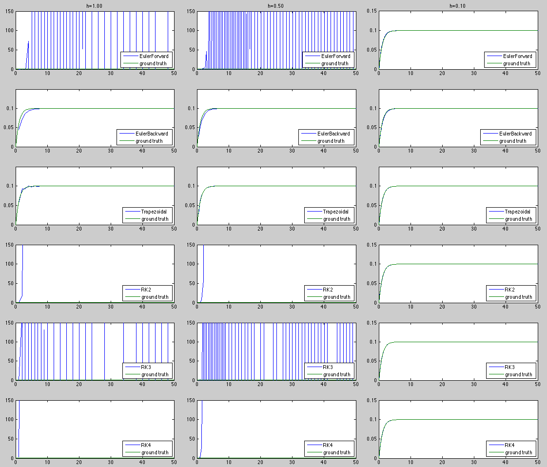
In the first case $s_1$ and $s_2$ are a complex conjugate pair, the system is underdamped. But in all other cases, both $s_1$ and $s_2$ are real, the system is overdamped, its solution contains two exponentially decaying terms $c_1 e^{s_1t}$ and $c_2 e^{s_2t}$, one decaying more quickly than the other.

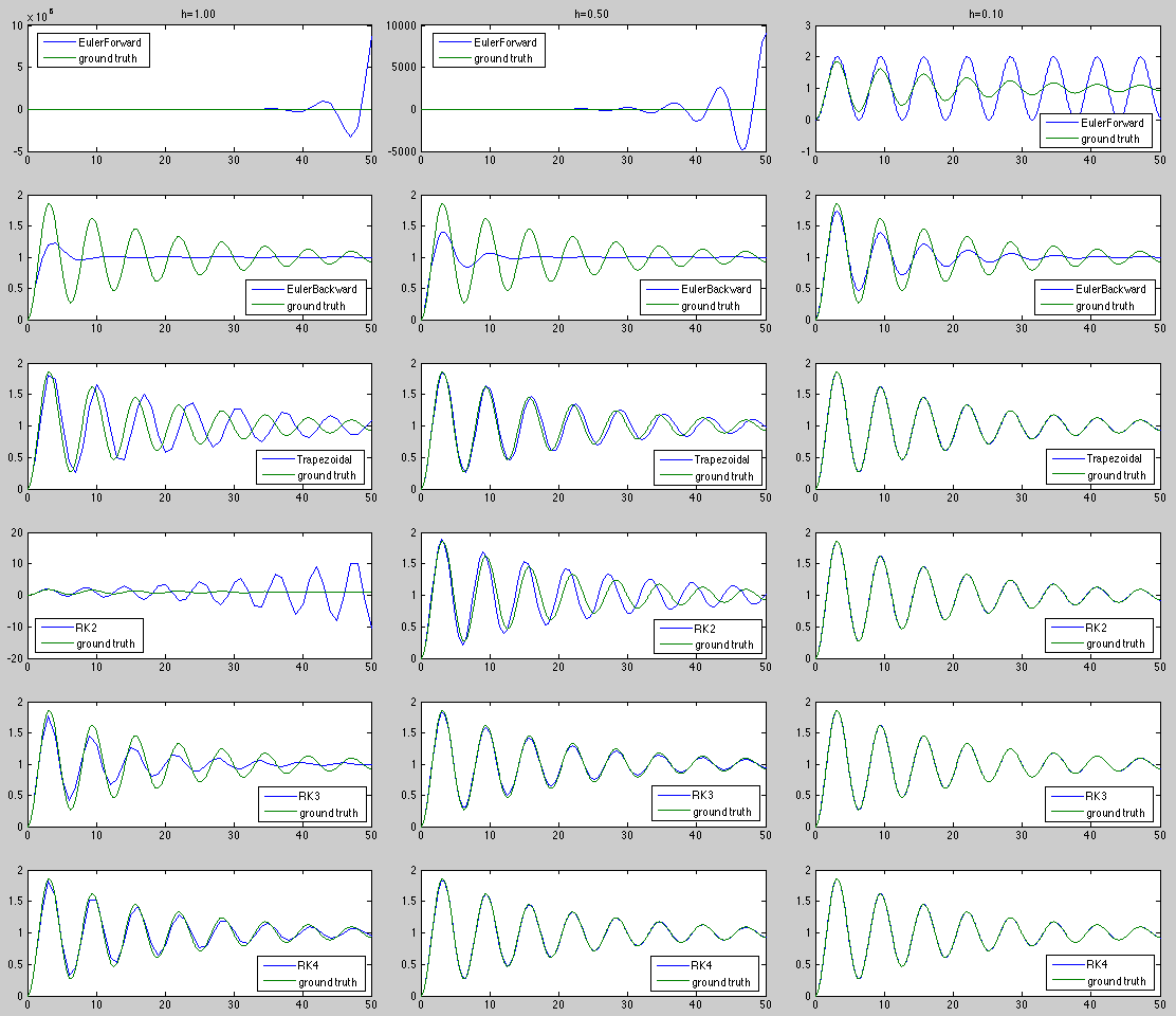
The numerical solutions are plotted together with the closed-form solution as the ground truth as show below.

• Case 1: step size $h=1$ (left), $h=0.5$ (middle), and $h=0.1$ (right)

  

• Case 2: The numerical solutions are shown below. We see that the implicit backward Euler and trapezoidal methods are always stable, but all other methods are not stable, i.e., their solutions grow without bound, if the step size is too small ($h=1$ or $h=0.5$).

  

• Case 3: The implicit backward Euler and trapezoidal methods are always stable, but all other methods are not stable, if the step size is less than $h=0.02$.

• Case 4: The two implicit method are always stable. The RK3 and RK4 are stable only if the step size is reduced to $h=0.003$, while the forward Euler and RK2 become stable only when the step size is further reduced to $h=0.002$.

Summarizing the above, we can make the following observations:

• A smaller step size always produces a more accurate soluton.
• Methods with higher order error terms are more accurate, if they are stable.
• When the ratio $Re(s_1)/Re(s_2)$ increases, a method may become unstable, the step size needs to be reduced to avoid a divergent solution.
• When the step size is not small enough, an explicit method may become not only inaccurate, but also unstable. A method of lower error order (forward Euler with $O(h^2)$, RK2 with $O(h^3)$) requires a smaller step size to remain stable than a method of higher error order (RK4 with $O(h^5)$).
• Small step size may be needed not necessarily for more accurate solution, but for preventing instability.
• The implicit backward Euler and trapezoidal methods are always stable even when the step size is large, although the orders of their error terms are not as high as other methods such as RK3 and RK4.
• A method with higher order error may produce more accurate solution only if it is stable, an implicit method with low error order may not be as accurate, but it is always stable.
• Accuracy and stability are two related but different properties of a method.

The Matlab code for the RK methods is listed below:

function RungeKutta
    global M C K
    M=10; C=1; K=10;
    
    figure(1)
%    M=1; C=101; K=100;   %stiff!
%    M=1; C=1001; K=1000;   %stiff!
    t0=0;                       % initial time
    y_int=[1; 1];               % initial values
    tfinal = 50;
    fprintf('Initial and final time:    %.2f to %.2f\n',t0,tfinal);
%    nsteps=input('Number of steps for numerical integral: ');

    
    for l=1:3
        switch l
            case 1
                nsteps=40;
            case 2
                nsteps=60;
            case 3
                nsteps=80;
        end
        tout=zeros(nsteps,1);
        h = (tfinal - t0)/ nsteps;       % step size
        
        y1=ones(nsteps,1);
        y2=ones(nsteps,1);
        y3=ones(nsteps,1);
        y4=ones(nsteps,1);
        y5=ones(nsteps,1);

        fprintf('\n# of steps: %4d\th=%0.3f\n',nsteps,h); 
        for k=0:4
            t = t0;                         % set the variable t.
            y = y_int;                      % initial conditions            
            for j= 1 : nsteps               % go through the steps.
                switch k
                    case 0        
                        y = EulerForward(h, t, y);
                        y1(j)=y(1);          % save only the first component of y.
                    case 1
                        %y=modifiedEuler(h, t, y);
                        y=EulerBackward(h, t, y);
                        y2(j)=y(1);
                    case 2
                        y=RungeKutta2(h, t, y);
                        y3(j)=y(1);
                    case 3
                        y=RungeKutta3(h, t, y);
                        y4(j)=y(1);
                    case 4
                        y=RungeKutta4(h, t, y, 3);
                        y5(j)=y(1);
                end
                t = t + h;      
                tout(j) = t;
            end
        end
        y0=SecondOrder(y_int,tout);

        subaxis(5,3,l, 'Spacing', 0.04, 'Padding', 0, 'Margin', 0.05);
        plot(tout,y0,tout,y1)
        xlim([t0,tfinal])        
%        ylim([-10 100])
        legend('ground truth','EulerForward')        
        fprintf('\tEulerForward:\terror=%e\n',norm((y0-y1)./y0)/nsteps)
        
        str = sprintf('h=%.2f',h);
        title(str);
        subaxis(5,3,l+3, 'Spacing', 0.04, 'Padding', 0, 'Margin', 0.05);
        plot(tout,y0,tout,y2)
        xlim([t0,tfinal])
%        ylim([-10 100])
        legend('ground truth','EulerBackward')
        fprintf('\tEulerBackward:\terror=%e\n',norm((y0-y2)./y0)/nsteps)
        
        subaxis(5,3,l+6, 'Spacing', 0.04, 'Padding', 0, 'Margin', 0.05);
        plot(tout,y0,tout,y3)
        xlim([t0,tfinal])
%        ylim([-10 100])
        legend('ground truth','RK2')
        fprintf('\tRK2:\terror=%e\n',norm((y0-y3)./y0)/nsteps)
        
        subaxis(5,3,l+9, 'Spacing', 0.04, 'Padding', 0, 'Margin', 0.05);
        plot(tout,y0,tout,y4)
        xlim([t0,tfinal])
%        ylim([-10 100])
        legend('ground truth','RK3')
        fprintf('\tRK3:\terror=%e\n',norm((y0-y4)./y0)/nsteps)
        
        subaxis(5,3,l+12, 'Spacing', 0.04, 'Padding', 0, 'Margin', 0.05);
        plot(tout,y0,tout,y5)
        xlim([t0,tfinal])
%        ylim([-10 100])
        legend('ground truth','RK4')
        fprintf('\tRK4:\terror=%e\n',norm((y0-y5)./y0)/nsteps)

    end
end

function e=rr(x,y)    
    e=0;    
    for i=1:length(x)
        e=e+abs(x(i)-y(i))/abs(y(i));        
    end
%     e=sqrt(e)
%     norm(x-y)
%     pause
end

function y = SecondOrder(y_int,t)
    global M C K
    zt=C/2/sqrt(M*K);
    wn=sqrt(K/M);
    s=sqrt(zt^2-1);
    s1=(-zt-s)*wn;
    s2=(-zt+s)*wn;
    c1=(s2*y_int(1)-y_int(2))/(s2-s1);
    c2=(s1*y_int(1)-y_int(2))/(s1-s2);
    y=c1*exp(s1*t)+c2*exp(s2*t);    % homogeneous solution
    y=y+1/(M*wn^2);                 % particular solution
end


function dy = f(t, y)    % 2nd order linear constant-coefficient DE
    global M C K
    dy = zeros(2,1);
    dy(1) = y(2);
    dy(2) = (-C*y(2)-K*y(1))/M;     % homogeneous solution
    dy(2) = dy(2)+1/M;              % particular solution
end


function y = EulerForward(h, t, y)
    y = y + h* f(t, y);
end

function y1 =  EulerBackward(h, t0, y0)    
    global M C K
    Jf=zeros(2);
    Jf(1,1)=0;
    Jf(1,2)=1;
    Jf(2,1)=-K/M;
    Jf(2,2)=-C/M;
    y1=y0;
    f(t0,y1);
    F=y0+h*f(t0,y1)-y1;
    norm(F);
    i=0;
    while norm(F)>0.0001  
        Jy=h*Jf;
        Jy(1,1)=Jy(1,1)-1;
        Jy(2,2)=Jy(2,2)-1;
        y1=y1-inv(Jy)*F;
        F=y0+h*f(t0,y1)-y1;
        norm(F);
    end
end


function y = modifiedEuler(h, t, y)
    k1 = f(t, y);
    k2 = f(t+h, y + h*k1);
    y = y + h*(k1 + k2)/2; 
end

function y = RungeKutta2(h, t, y)
    k1 = f(t, y);
    k2 = f(t+h/2, y + h*k1/2);
    y = y + h*k2;
end

function y = RungeKutta3(h, t, y)
     k1 = f(t, y);
     k2 = f(t+h/2, y + h*k1/2);
     k3 = f(t+h, y -h*k1 + 2*h*k2);
     y = y + h*(k1 + 4*k2 + k3)/6;
%    k1 = f(t0, y0);
%    k2 = f(t0+h/3, y0 + h*k1/3);
%    k3 = f(t0+2*h/3, y0 +2*h*k2/3);
%    y1 = y0 + h*(k1 + 3*k3)/4;
end

function y1 = RungeKutta2a(h, t0, y0)
    a=0.5;
    k1 = f(t0, y0);
    k2 = f(t0+a*h, y0 + a*h*k1);
    y1 = y0 + h*((1-1/2/a)*k1+ k2/2/a)/2;
end


function y = RungeKutta4(h, t, y, k)
    k1 = f(t, y);
    switch k
        case 1
            k2 = f(t+h/2, y + h*k1/2);    
            k3 = f(t+h/2, y + h*k2/2);
            k4 = f(t+h, y + h*k3);
            y  = y + h*(k1 + 2*k2 + 2*k3 + k4)/6;
        case 2
            k2 = f(t+h/3, y + h*k1/3);
            k3 = f(t+2*h/3, y -h*k1/3 +h*k2);
            k4 = f(t+h, y + h*k1 -h*k2 +h*k3);
            y  = y + h*(k1 + 3*k2 + 3*k3 + k4)/8;
        case 3
            k2 = f(t+2*h/3, y + 2*h*k1/3);
            k3 = f(t+h/3, y + h*k1/12 +h*k2/4);
            k4 = f(t+h, y - 5*h*k1/4 +h*k2/4 +2*h*k3);
            y  = y + h*(k1 + 3*k2 + 3*k3 + k4)/8;
        case 4
             k2 = f(t+h/2, y + h*k1/2);
             k3 = f(t+h/2, y + h*k1/6 +h*k2/3);
             k4 = f(t+h, y -h*k2/2 +3*h*k3/2);
             y  = y + h*(k1 + k2 + 3*k3 + k4)/6;
        case 5
            k2 = f(t+h/2, y + h*k1/2);
            k3 = f(t+h/2, y - h*k1/2 +h*k2);
            k4 = f(t+h, y + h*k2/2 + h*k3/2);
            y  = y + h*(k1 + 3*k2 + k3 + k4)/6;
    end    
end