Euler's methods

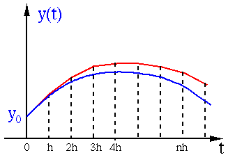
The slope of the secant through $y(t)$ and $y(t+h)$ can be approximated by $y'(t)$, $y'(t+h)$, or, more accurately, the average of the two: $(y'(t)+y'(t+h))/2$. Correspondingly, we have the following three methods:

• Forward Euler's method:

  This method uses the derivative $y'(t)$ at the beginning of the interval $[t,\;t+h]$ to approximate the increment $\Delta y\approx h\,y'(t)$:

  $$\hat{y}(t+h)=y(t)+h\,y'(t)=y(t)+h\,f(t,y(t))$$ (189)

  Comparing this method with the Taylor series expansion of $y(t+h)$:

  $$y(t+h)=y(t)+y'(t)\;h+\frac{y''(t)}{2}h^2+\frac{y'''(t)}{3!}h^3+\cdots$$ (190)

  we see that this method has a second order truncation error $O(h^2)$.

  If the step size $h$ is not small enough, this truncation error will accumulate as the iterative process progresses, and $y_n$ so generated may deviate from the true solution $y(t)$ quickly in a few steps. Consequently, the iteration may become divergent $y_n\rightarrow \pm\infty$, i.e., the method may not be stable. Therefore Euler's method is useful only if the step size $h$ is sufficiently small, so that the error does not accumulate too quickly.

  

• Backward Euler's method:

  This method uses the derivative $y'(t+h)$ at the end of the interval $[t,\;t+h]$ to approximate the increment $\Delta y\approx h\,y'(t)$:

  $$\hat{y}(t+h)=y(t)+h\,y'(t+h) = y(t)+h\,f(t+h,y(t+h))$$ (191)

  Replacing $y'(t+h)$ in the expression by its Taylor expansion:

  $$y'(t+h)=y'(t)+h y''(t)+\frac{h^2}{2}y'''(t)+O(h^3)$$ (192)

  we get

  $$\hat{y}(t+h) \approx y(t)+h\,y'(t+h)=y(t)+h y'(t)+h^2 y''(t)+O(h^3)$$ (193)

  Comparing this with the Taylor expansion in Eq. (190), we see that the backward Euler's method also has a second order error $O(h^2)$. As the desired function value $y(t+h)$ appears on both sides of Eq. (191), this method is implicit, instead of explicit, as $y(t+h)$ needs to be found by solving the following equation for $x=y(t+h)$ treated as the unknown:

  $$F(x)=y(t)+h\,f(t+h, x)-x=0$$ (194)

  In general, the Newton-Raphson method can be used to solve this equation by the following iteration from some initial guess $x_0$:

  $$x_{n+1}=z_n-\frac{F(x)}{F'(x)} \;\;\;\;\;\; \;\;\;\;\;\; F'(x)=\frac{d}{dx}F(x)=h\,\frac{df(t+h, x)}{dx}-1$$ (195)

  Obviously this method is more computationally expensive, however, as an implicit method, it is always stable compared to the forward method, as shown below.

• Trapezoidal method (Heun's method):

  This method uses the average of the derivatives at the beginning and end points of the interval $[t,\;t+h]$ as an estimate of the slope of the secant:

  $$y'(t+ch)\approx \frac{y'(t)+y'(t+h)}{2}$$ (196)

  so that the next function value can be approximated as
  

  $$y(t+h)=y(t)+h\,y'(t+ch)\approx y(t)+h\,\frac{y'(t)+y'(t+h)}{2}$$

  $$=y(t)+\frac{h}{2}\,[f(t,\,y(t))+f(t+h,\,y(t+h))]$$ (197)

  
  which can also be obtained by applying the trapezoidal rule of the Newton-Cotes quadrature to approximate the integral in the iteration:
  

  $$y(t+h) = y(t)+\int_t^{t+h} y'(\tau)\,d\tau =y(t)+\frac{h}{2}\,[y'(t)+y'(t+h)]$$

  $$= y(t)+\frac{h}{2}\,[f(t,\,y(t))+f(t+h,\,y(t+h))]$$ (198)

  
  This can be expressed iteratively:

  $$y_{n+1}=y_n+\frac{h}{2}[ f(t_n,\,y_n)+f(t_n+h,\,y_n+hf_n) ] =y_n+h\left(\frac{1}{2}k_1+\frac{1}{2}k_2\right)$$ (199)

  where

  $$\left\{ \begin{array}{l}k_1=f(t_n,y_n)=f_n \\ k_2=f(t_n+h,\,y_n+hk_1)\end{array}\right.$$ (200)

  

  To find the order of the truncation error, we replace $y'(t+h)$ in the equation by its Taylor expansion $y'(t+h)=y'(t)+h y''(t)+O(h^2)$ and rewrite the equation above as
  

  $$\hat{y}(t+h) = y(t)+\frac{h}{2}\,y'(t)+\frac{h}{2}\,y'(t+h)$$

  $$= y(t)+\frac{h}{2}\,y'(t)+\frac{h}{2}\,[y'(t)+h y''(t)+O(h^2)]$$

  $$= y(t)+h\,y'(t)+\frac{h^2}{2} y''(t)+O(h^3)$$ (201)

  
  Comparing this with the Taylor expansion in Eq. (190), we see that the trapezoidal method has a third order error $O(h^3)$, one order higher than either the forward or backward method.

  Same as the backward method, this traperoidal method is also implicit. To find $x=y(t+h)$, we need to solve the following equation:

  $$F(x)=y(t)+\frac{h}{2}f(t,\,y(t))+\frac{h}{2} f(t+h,\,x)-x=0$$ (202)

In summary, here is how the three methods find the increment of function $y(t)$:

$$\Delta y =h\,f'(t+ch) \approx h\,\left\{\begin{array}{ll} y'(t) & O(h^2) \\ y'(t+h) & O(h^2) \\ (y'(t)+y'(t+h))/2 & O(h^3) \end{array}\right.$$ (203)

which can be implemented iteratively from the known initial condition $y_0=y(0)$

$$y_{n+1}=y_n+h\,\left\{\begin{array}{l} y'_n \\ y'_{n+1} \\ (y'_n+... ...n)\\ f(t_{n+1},y_{n+1})\\ (f(t_n,y_n)+f(t_{n+1},y_{n+1}))/2 \end{array}\right.$$ (204)

Example: Consider a simple first order constant coefficient DE:

$$y'(t)+\lambda y(t)=0,\;\;\;\;\; \;\;\;\;\;\; y'(t)=f(t,\,y(t))=-\lambda y(t)$$ (205)

with $\lambda>0$ and initial condition $y(0)=y_0$. The closed form solution of this equation is known to be $y(t)=y_0 e^{-\lambda t}$, which decays exponentially to zero when $t\rightarrow \infty$. This DE can be solved numerically by each of the three methods.

• The forward Euler's method:
  

  $$y_{n+1} = y_n+h\,f(t_n,y_n)=y_n-\lambda h\, y_n=(1-\lambda h) y_n$$

  $$= (1-\lambda h)^2 y_{n-1}=\cdots =(1-\lambda h)^{n+1} y_0$$ (206)

  
  The iteration will converge to the solution, only if $\vert 1-\lambda h\vert<1$ i.e., $0<\lambda h<2$ or $h<2/\lambda$. If the step size is greater than $2/\lambda$, iteration will diverge.
• The backward Euler's method:

  $$y_{n+1}=y_n+h\,f(t_{n+1},y_{n+1})=y_n- \lambda h y_{n+1}$$ (207)

  Solving the equation for $y_{n+1}$ we get

  $$y_{n+1}=\frac{y_n}{1+\lambda h}$$ (208)

• The trapezoidal method:

  $$y_{n+1}=y_n+h\,\frac{f(t_n,y_n)+f(t_{n+1},y_{n+1})}{2} =y_n- \lambda h\frac{y_n+y_{n+1}}{2}$$ (209)

  Solving the equation for $y_{n+1}$ we get

  $$y_{n+1}=\frac{2-\lambda h}{2+\lambda h}\,y_n$$ (210)

The results of all three methods are shown together with the ground truth solution $y(t)=y_0 e^{-\lambda t}$ with $y_0=1$ and $\lambda=1$. The four plots correspond to five different step sizes $h=0.5,\;0.83,\;1.67,\;2.0,\;2.2$.

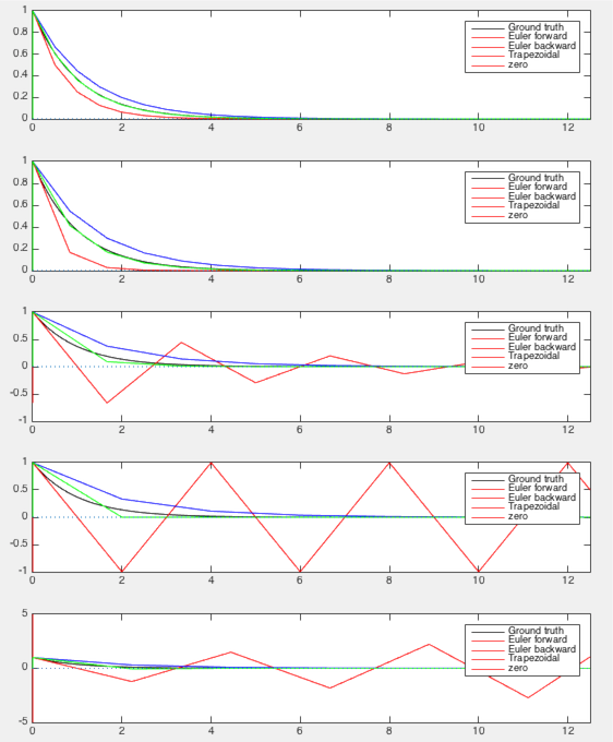
We make the following observations:

• The solution of the forward method is always below the true solution, while that of the backward method is always above. This is because the negative slop of the solution, whose magnitude is continuously reduced, is over estimated by $y'_n$ used in the forward method, but under estimate by $y'_{n+1}$ used by the backward method. As the average of the two, the result of the trapezoidal method coincide with the true solution more closely.
• The backward method always produces a stable approximation of the function $y(t)$, while the performance of the forward method is very sensitive to the step size $h$. In particular, when $h>2/\lambda=2$, the iteration becomes divergent.

In general there are two different types of approaches to estimate some value in the future, such as the next function value $y_{n+1}=y(t+h)$:

• Explicit methods are based on the present and past information, such as $y_n$ and $y_{n-1}$. Such a method may be divergent and therefore unstable (the iteration grows out of bound);
• Implicit methods are based on some unknown information in the future, such as $y_{n+1}$, as well as the present and past information such as $y_n$ and $y_{n-1}$. Such a method is in general stable.

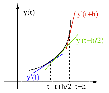
We further consider the Midpoint method which uses the midpoint $y(t+h/2)$ between the two end point $y(t)$ and $y(t+h)$. Consider the Taylor series expansion of $y(t+h)$:

$$y(t+h)=y(t)+y'(t)h+\frac{h^2}{2!}y''(t)+\frac{h^3}{3!}y'''(t)+O(h^4)$$ (211)

which can be rewritten as the following:

$$\frac{y(t+h)-y(t)}{h}=y'(t)+\frac{h}{2}y''(t)+\frac{h^2}{6}y'''(t)+O(h^3)$$ (212)

On the other hand, the Taylor series for $y'(t+h/2)$ is:

$$y'\left(t+\frac{h}{2}\right)=y'(t)+\frac{h}{2}y''(t)+\frac{h^2}{8}y'''(t)+O(h^3)$$ (213)

The difference between these two equations above is:

$$\frac{y(t+h)-y(t)}{h}-y'\left(t+\frac{h}{2}\right)=O(h^2)$$ (214)

Solving for $y(t+h)$ we get

$$y(t+h)=y(t)+h\, y'\left(t+\frac{h}{2}\right)+h\,O(h^2) =y(t)+h f\left(t+\frac{h}{2},\,y\left(t+\frac{h}{2}\right)\right) +O(h^3)$$ (215)

The third order error term $O(h^3)$ is one order higher than that of either Euler's forwar or backward method. This equation can be expressd iteratively:

$$y_{n+1}=y_n+h f\left(t_n+\frac{h}{2},\,y\left(t_n+\frac{h}{2}\right)\right)$$ (216)

The second argument $y(t_n+h/2)$ of the function on the right-hand side can be approximated by the first two terms of its Taylor expansion:

$$y\left(t_n+\frac{h}{2}\right)\approx y(t_n)+\frac{h}{2}y'(t_n) =y_n+\frac{h}{2}f(t_n,\,y_n)=y_n+\frac{h}{2}f_n$$ (217)

Substituting this back into the iteration above we get:

$$y_{n+1}=y_n+h f\left(t_n+\frac{h}{2},y_n+\frac{h}{2}f_n\right) =y_n+h f\left(t_n+\frac{h}{2},\,y_n+\frac{h}{2}k_1 \right) =y_n+hk_2$$ (218)

where

$$\left\{ \begin{array}{l} k_1=f(t_n,\,y_n)=f_n\\ k_2=f(t_n+\frac{h}{2},y_n+\frac{h}{2}k_1)\end{array}\right.$$ (219)