Newton-Cotes Quadrature

Here we assume the $n+1$ sample points of the integrand $f(x)$ are equally spaced:

$$x_{i+1}-x_i=h=\frac{b-a}{n},\;\;\;\;\;\;(i=0,\cdots,n-1)$$ (28)

then we have $x_0=a,\;\;\;x_i=a+ih,\;\;\;x_n=a+nh=b$. We further introduce another variable $t$ so that $x=a+th$, and $dx=h\,dt,\;\;\;\;x-x_j=(t-j)h$, and the coefficients in Eq. (25) can be written as:

$$c_i = \int_a^b\left(\prod_{j=0,\;j\ne i}^n \frac{x-x_j}{x_i-x_j}\right)dx =\int_0^n \left(\prod_{j=0,\;j\ne i}^n\frac{t-j}{i-j}\right)\,h\,dt$$

$$= h\int_0^n \frac{\prod_{j=0,\;j\ne i}^n (t-j)} {i(i-1)\cdots(i-i+1)\;(i-i-1)\cdots(i-n)} dt$$

$$= h\;\frac{(-1)^{n-i}}{i!\,(n-i)!}\int_0^n \frac{\prod_{j=0}^n(t-j)}{t-i}\;dt,\;\;\;\;\;\;(i=0,\cdots,n)$$ (29)

These $n+1$ coefficients can be found by the following Matlab:

function c=coefs(n)
    syms x
    w=1;
    for i=0:n
        w=w*(x-i);
    end
    c=[];
    for i=0:n        
        f=w/(x-i);
        ci=int(f,[0,n])*(-1)^(n-i)/factorial(i)/factorial(n-i);
        c=[c ci];
    end
end

This integral of an nth-degree polynomial can be easily carried out. The quadrature rule based on such coefficients is called the Newton-Cotes formula:

$$I_n[f]=\sum_{i=0}^n c_i\;f(x_i)=\sum_{i=0}^n c_i\;y_i$$ (30)

As mentioned before, in general the degree of accuracy of $I_n[f]$ is at least $n$. We now further show that if the sample points are equally spaced and if $n$ is even, the degree of accuracy of $I_n[f]$ is at least $n+1$. Consider a polynomial integrand of degree $n+1$, e.g., $f(x)=x^{n+1}$. We have $f^{(n+1)}(x)=(n+1)!$ and the integration error is

$$E_n[x^{n+1}] = \int_a^b R_n(x)dx=\frac{1}{(n+1)!} \int_a^b f^{(n+1)}(\xi)\prod_{i=0}^n(x-x_i)dx$$

$$= \int_a^b \prod_{i=0}^n(x-x_i)dx=h^{n+2}\int_0^n \prod_{i=0}^n(t-i)dt$$ (31)

Since $n$ is even, $n/2$ is an integer. Introducing $u=t-n/2$, we further get

$$E_n[x^{n+1}]=h^{n+2}\int_{-n/2}^{n/2} \prod_{i=0}^n(u-i+n/2)\, du =h^{n+2}\int_{-n/2}^{n/2} \prod_{j=-n/2}^{n/2}(u-j)\, du=0$$ (32)

The last equation is due to the fact that the integrand is an odd function of $u$. This result indicates that when $n$ is even, the degree of accuracy of $I_n[f]$ is at least $n+1$.

Given the integrand $f(x)$ and the quadrature rule, we need to further determine the specific integration error

$$E_n[f]=\int_a^b R_n(x)\,dx =\int_a^b\frac{f^{(n+1)}(\xi(x))}{(n+1)!}l_n(x)\,dx$$ (33)

If $l_n(x)$ does not change sign in the interval $(a,\,b)$, we can further have

$$E_n[f]=\frac{f^{(n+1)}(\eta)}{(n+1)!}\int_a^b l_n(x)\,dx$$ (34)

according to the weighted mean-value theorem for integrals, where $\eta\in [a,\,b]$. However, if $l_n(x)$ does change signs in the interval, this result is not valid and we have to try some other method. In this case, we assume the integration error takes the form $E_n[f]=Kf^{(m+1)}(\eta)$, where $K$ is a constant independent of $f(x)$, if the degree of accuracy of $L_n(x)$ is $m$. This way, $E_n[x^k]=K\,(x^k)^{(m+1)}$ is zero if $k\le m$ but non-zero if $k>m$, i.e., the degree of accuracy of $L_n(x)$ is indeed $m$. Next, to find $K$, we let $f(x)=x^{m+1}$ with $f^{(m+1)}(x)=(m+1)!$, and get

$$K=\frac{E_n[f]}{f^{(n+1)}(x)}=\frac{E_n[x^{m+1}]}{(x^{m+1})^{(m+1)}} =\frac{E_n[x^{m+1}]}{(m+1)!}$$ (35)

Now the integration error can be found to be

$$E_n[f]=K f^{(m+1)}(\eta) =\frac{f^{(m+1)}(\eta)}{(m+1)!}E_n[x^{m+1}] =\frac{f^{(m+1)}(\eta)}{(m+1)!}\int_a^b l_m(x)dx$$ (36)

The last equation is due to Eq. (?) in the previous section, where $E_n[x^{m+1}]$ can be found by either of two ways:

$$E_n[x^{m+1}] = I[x^{m+1}]-I_n[x^{m+1}]$$

$$= \int_a^b l_m(x)dx=\int_a^b \prod_{i=0}^m(x-x_i)\,dx =h^{n+2}\int_0^n t(t-1)\cdots(t-m)\,dt$$ (37)

In the following, we will consider the Newton-Cotes quadrature and its integration error for $n=1,\;2,\;3,\;4$.

• $n=1$ based on $n+1=2$ points, the trapezoidal rule:

  $$h=b-a,\;\;x_0=a,\;x_1=a+h=b$$ (38)

  
  

  $$c_0 = -h\int_0^1 (t-1)\,dt=\frac{h}{2}$$

  $$c_1 = h\int_0^1 t\, dt=\frac{h}{2}$$ (39)

  
  The trapezoidal rule is:

  $$I_1[f]=c_0 f(x_0)+c_1 f(x_1)=\frac{h}{2}(f(x_0)+f(x_1))$$ (40)

  To find the degree of accuracy, considering the follwoing polynomial integrands:
  • $f(x)=x^n=x$:
    

    $$I[x] = \int_a^b x\,dx=\frac{b^2-a^2}{2}$$

    $$I_1[x] = \frac{b-a}{2}(a+b)=\frac{b^2-a^2}{2}$$ (41)

    
    

    $$E_1[x]=I[x]-I_1[x]=0$$ (42)

  • $f(x)=x^{n+1}=x^2$:
    

    $$I[x^2] = \int_a^b x^2\, dx=\frac{b^3-a^3}{3}$$

    $$I_1[x^2] = \frac{b-a}{2}(a^2+b^2)\ne I[x^2]$$ (43)

    
    

    $$E_1[x^2]=I[x^2]-I_1[x^2]=-\frac{(b-a)^3}{6} =-\frac{h^3}{6}\ne 0$$ (44)

    $E_1[x^2]$ can also be obtained as:

    $$E_1[x^2]=\int_a^b l_1(x)\,dx=h^3\int_0^1 t(t-1)\,dt =-\frac{h^3}{6}$$ (45)

  As $E_1[x^2]\ne 0$, the degree of accuracy of $I_1[f]$ is $m=1=n$. The general integration error is:

  $$E_1[f]=\frac{f''(\eta)}{2} E_1[x^2]=-\frac{h^3}{12}f''(\eta) =\frac{(b-a)^3}{12}f''(\eta)$$ (46)

• $n=2$ based on $n+1=3$ points, Simpson's rule:

  $$h=\frac{b-a}{2},\;\;x_0=a,\;\;x_1=\frac{a+b}{2},\;\;x_2=b$$ (47)

  
  

  $$c_0 = \frac{h}{2}\int_0^2 (t-1)(t-2)\,dt=\frac{h}{3}$$

  $$c_1 = -h\int_0^2 t(t-2)\, dt=\frac{4h}{3}$$

  $$c_2 = \frac{h}{2} \int_0^2 t(t-1)\,dt=\frac{h}{3}$$ (48)

  
  The Simpson's rule is:

  $$I_2[f]=c_0 f(x_0)+c_1 f(x_1)+c_2 f(x_2)=\frac{h}{3}(f(x_0)+4f(x_1)+f(x_2))$$ (49)

  To find the degree of accuracy, considering the follwoing polynomial integrands:
  • $f(x)=x^n=x^2$:
    

    $$I[x^2] = \int_a^b x^2\, dx=\frac{b^3-a^3}{3}$$

    $$I_2[x^2] = \frac{b-a}{6}\left[a^2+4\left(\frac{a+b}{2}\right)^2+b^2\right] =\frac{b^3-a^3}{3}$$ (50)

    
    

    $$E_2[x^2]=I[x^2]-I_2[x^2]=0$$ (51)

  • $f(x)=x^{n+1}=x^3$:
    

    $$I[x^3] = \int_a^b x^3\,dx=\frac{b^4-a^4}{4}$$

    $$I_2[x^3] = \frac{b-a}{6}\left[a^3+4\left(\frac{a+b}{2}\right)^3+b^3\right] =\frac{b^4-a^4}{4}$$ (52)

    
    

    $$E_2[x^3]=I[x^3]-I_2[x^3]=0$$ (53)

  • $f(x)=x^{n+2}=x^4$:
    

    $$I[x^4] = \int_a^b x^4\,dx=\frac{b^5-a^5}{5}$$

    $$I_2[x^4] = \frac{b-a}{6}\left[a^4+4\left(\frac{a+b}{2}\right)^4+b^4\right] =\frac{b-a}{24}(5a^4+4a^3b+6a^2b^2+4ab^3+5b^4)$$ (54)

    
    

    $$E_2[x^4]=I[x^4]-I_2[x^4]=-\frac{(b-a)^5}{120}=-\frac{4h^5}{15}$$ (55)

    $E_2[x^4]$ can also be obtained as:

    $$E_2[x^4]=\int_a^b l_3(x)\,dx=h^4\int_0^2 t(t-1)(t-2)(t-3)\,dt =-\frac{4h^5}{15}$$ (56)

  As $E_2[x^4]\ne 0$, the degree of accuracy of the Simpson's rule is $m=3=n+1>n$ ($n$ is even). The general integration error is:

  $$E_2[f]=\frac{f^{(4)}(\eta)}{4!}E_2[x^4] =-\frac{h^5}{90}f^{(4)}(\eta)=-\frac{(b-a)^5}{2880}f^{(4)}(\eta)$$ (57)

• $n=3$ based on $n+1=4$ points, Simpson's 3/8 rule:

  $$h=\frac{b-a}{3},\;\;x_0=a,\;\;x_1=\frac{2a+b}{3},\;\; x_2=\frac{a+2b}{3},\;\;x_3=b$$ (58)

  
  

  $$c_0 = -\frac{h}{3!}\int_0^3 (t-1)(t-2)(t-3)\,dt =\frac{3h}{8}$$

  $$c_1 = \frac{h}{2}\int_0^3 t(t-2)(t-3)\,dt=\frac{9h}{8}$$

  $$c_2 = -\frac{h}{2}\int_0^3 t(t-1)(t-3)\,dt=\frac{9h}{8}$$

  $$c_3 = \frac{h}{3!}\int_0^3 t(t-1)(t-2)\,dt=\frac{3h}{8}$$ (59)

  
  The quadrature rule is:

  $$I_3[f]=c_0f(x_0)+c_1f(x_1)+c_2f(x_2)+c_3f(x_3) =\frac{3h}{8}(f(x_0)+3f(x_1)+3f(x_2)+f(x_3))$$ (60)

  The degree of accuracy can be found by considering the follwoing polynomial integrands:
  • $f(x)=x^n=x^3$:
    

    $$I[x^3] = \int_a^b x^3\,dx=\frac{b^4-a^4}{4}$$

    $$I_3[x^3] = \frac{b-a}{8} \left[a^3+\frac{(2a+b)^3}{9} +\frac{(a+2b)^3}{9}+b^3\right]=\frac{b^4-a^4}{4}$$ (61)

    
    

    $$E_3[x^3]=I[x^3]-I_3[x^3]=0$$ (62)

  • $f(x)=x^{n+1}=x^4$:
    

    $$I[x^4] = \int_a^b x^4\,dx=\frac{b^5-a^5}{5}$$

    $$I_3[x^4] = \frac{b-a}{8} \left[a^4+3\left(\frac{2a+b}{3}\right)^4 +3\left(\frac{a+2b}{3}\right)^4+b^4\right]$$

    $$= \frac{1}{54}(-11a^5+a^4b-2a^3b^2+2a^2b^3-ab^4+11b^5)$$

    
    

    $$E_3[x^4]=I[x^4]-I_3[x^4]=-\frac{(b-a)^5}{270}=-\frac{9h^5}{10}$$ (63)

    $E_3[x^4]$ can also be obtained by:

    $$E_3[x^4]=\int_0^{3h} l_3(x)\,dx=h^5\int_0^3 t(t-1)(t-2)(t-3)\,dt =-\frac{9h^5}{10}$$ (64)

  As $E_3[x^4]\ne 0$, the degree of accuracy is $m=3=n$. The general integration error is:

  $$E_3[f]=\frac{f^{(4)}(\eta)}{4!}E_3[x^4] =-\frac{3\,h^5}{80}f^{(4)}(\eta)=\frac{(b-a)^5}{6480}f^{(4)}(\eta)$$ (65)

• $n=4$ based on $n+1=5$ points, Boole's rule:

  $$h=\frac{b-a}{4},\;\;x_0=a,\;\;x_1=\frac{3a+b}{4},\;\; x_2=\frac{2a+2b}{4},\;\;x_3=\frac{a+3b}{4},\;\;x+4=b$$ (66)

  The quadrature rule is:
  

  $$I_4[f] = c_0 f(x_0)+c_1 f(x_1)+c_2 f(x_2)+c_3 f(x_3)+c_4 f(x_4)$$

  $$= \frac{2h}{45}(7 f(x_0)+32 f(x_1)+12 f(x_2)+32 f(x_3)+7 f(x_4))$$ (67)

  
  

The coefficients and integration errors for other quadrature rules with higher $n$ can be similarly obtained.

$$\begin{array}{c\vert c\vert c\vert\vert r\vert r\vert r\vert ... ... 5/288 & 19 & 75 & 50 & 50 & 75 & 19 & & \\ \hline \end{array}$$

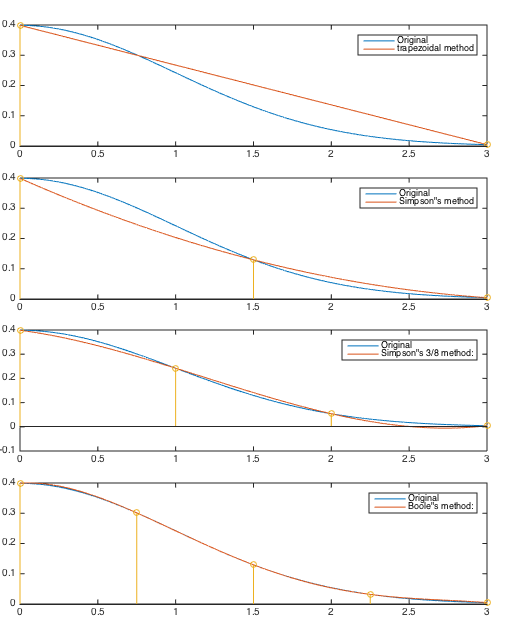
Example:

Here we consider the integral of the normal (Gaussian) distribution function with zero mean and unit standard deviation $\sigma=1$:

$$\int_0^3 g(x)\,dx=\frac{1}{\sqrt{2\pi}}\int_0^3 \exp\left(-\frac{x^2}{2}\right)\,dx$$ (68)

Twice of this value is the probability of $x$ taking a value within 3 standard deviations. This integral is carried out by each of the four methods with different truncation errors. We see that as $n$ increases, the error $E_n[g]$ reduces.

$$\begin{array}{c\vert\vert c\vert c\vert c\vert c}\hline n & 1... ....06e-01 & 3.79e-02 & 1.44e-02 & -2.35e-03 \\ \hline \end{array}$$ (69)