Phase Plane Portrait and Stability

Consider a first-order autonomous ODE system containing $N=2$ equations:

$${\bf y}'(t)={\bf f}(y_1,\;y_2), \;\;\;\;\;\; \;\;\;\;\;\;\;\; \left[\begin{array}{l} y_1'(t)\\ y_2'(t)\end{arr... ...right] =\left[\begin{array}{l}f_1(y_1,\;y_2)\\ f_2(y_1,\;y_2)\end{array}\right]$$ (155)

Note that the system is autonomous as it does not explicitly depends on the independent variable $t$. A phase plane plot can be made to visualize certain properties such as the stability of the solution. Specifically, let $y_1$ and $y_2$ span a 2-D plane in which every point is associated with a vector with two components

$${\bf f}=\left[\begin{array}{c}f_1\\ f_2\end{array}\right] =\left[\begin{array}{c}y'_1\\ y'_2\end{array}\right]$$ (156)

represented by an arrow indicating the direction along which the system is moving as time $t$ progresses. If the vector at a point is zero

$${\bf f}=\left[\begin{array}{l} f_1\\ f_2\end{array}\right] =\left[\begin{array}{l} 0\\ 0\end{array}\right]={\bf0}$$ (157)

then the point is an equalibrium point.

We first consider the special case of LCCODE as an example:

$${\bf y}'=\left[\begin{array}{c}y_1\\ y_2\end{array}\right]' =\lef... ... d\end{array}\right] \left[\begin{array}{c}y_1\\ y_2\end{array}\right]={\bf Ay}$$ (158)

Obviously the point $y_1=y_2=0$ is an equilibrium solution at which ${\bf y}'={\bf f}={\bf Ay}={\bf0}$. As the solution of this homogeneous system is in the following form:

$${\bf y}=c_1e^{\lambda_1t}{\bf v}_1+c_2e^{\lambda_2t}{\bf v}_2$$ (159)

we see that this solution is stable if the real parts of all eigenvalues are smaller than zero. By solving the characteristic equation of ${\bf A}$:

$$\det( \lambda{\bf I}-{\bf A} ) = \det \left[\begin{array}{cc}\lambda-a & -b\\ -c & \lambda-d\end{array}\right] =(\lambda-a)(\lambda-d)-bc$$

$$= \lambda^2-(a+d)\lambda+ad-bc =\lambda^2-T\lambda+D=0$$ (160)

where $T=tr({\bf A})=a+d$ and $D=det({\bf A})=ad-bc$ are the trace and determinant of ${\bf A}$ respectively, we can get the eigenvalues of ${\bf A}$

$$\lambda_{1,2}=\frac{1}{2}\left(T\pm\sqrt{T^2-4D}\right) =\frac{1}{2}\left(T\pm\sqrt{\Delta}\right)$$ (161)

where $\Delta=T^2-4D$.

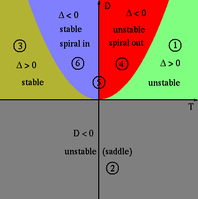
• If $D>T^2/4>0$ (above the parabola), i.e., $\Delta=T^2-4D<0$, then $\lambda_{1,2}=(T\pm j\sqrt{-\Delta})/2$ are two complex conjugate roots,

  $$\left\{\begin{array}{ll} T>0, & \mbox{unstable (spiral out)}\\ T... ...trally stable (marginal)}\\ T<0, & \mbox{stable (spiral in)}\end{array}\right.$$ (162)

• If $0<D<T^2/4$ (between the parabola and horizontal axis), i.e., $\Delta=T^2-4D>0$, then $\lambda_{1,2}=(T\pm \sqrt{\Delta})/2$ are two real roots,

  $$\left\{\begin{array}{ll} T>0, & \lambda_{1,2}>0, \mbox{unstable}\\ T<0, & \lambda_{1,2}<0, \mbox{stable}\end{array}\right.$$ (163)

• If $D<0$ (below horizontal axis), i.e., $\sqrt{T^2-4D}>T$, then $\lambda_{1,2}=(T\pm \sqrt{\Delta})/2$ have opposite signs, unstable (saddle point);

In summary, the solution is stable only if $T\le 0$ and $D>0$ (the top-left quadrant).

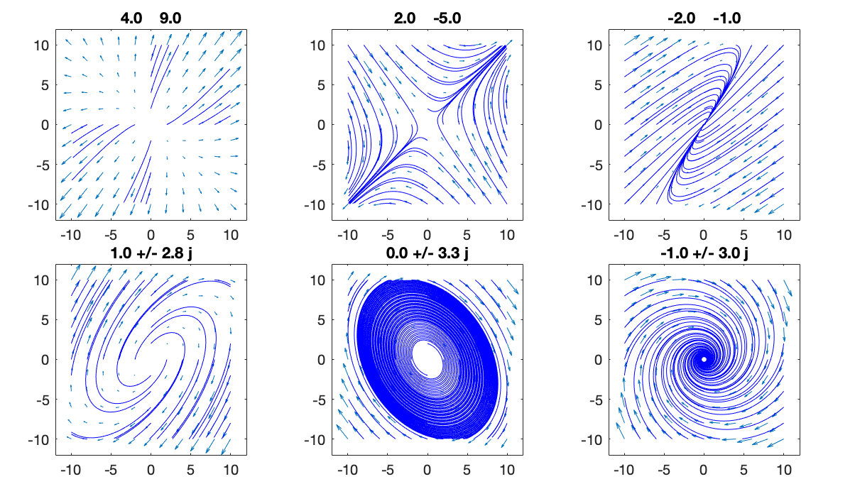
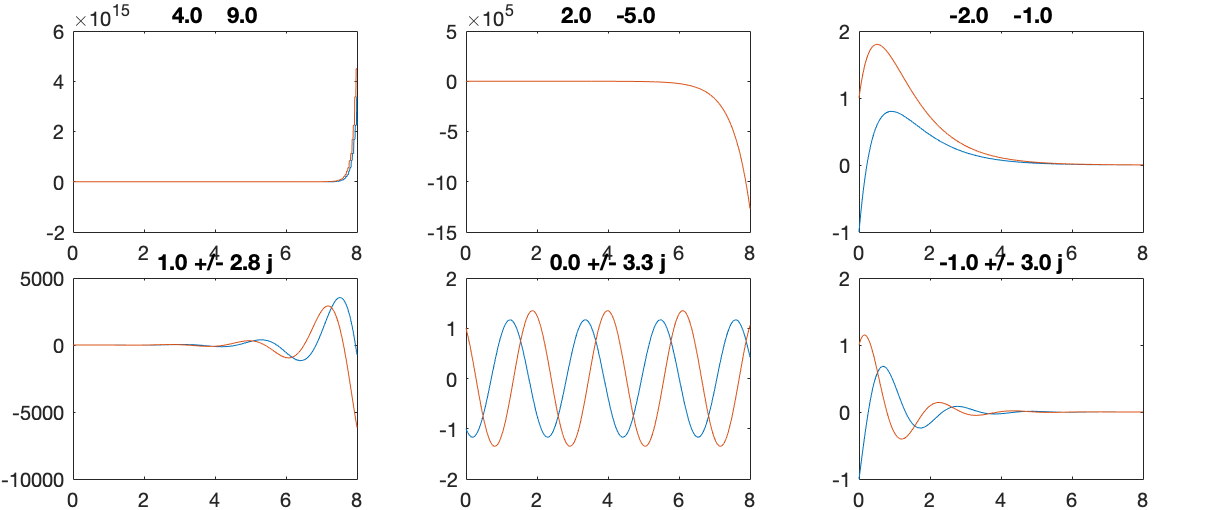
The behavior of the dynamic system described by a first order ODE system can be visualized by the phase plane portrait, in which the derivative ${\bf y}'=[y'_1,\;y'_2]$ at each point ${\bf y}=[y_1,\;y_2]^T$ is drawn as an arrow, as shown in the examples below:

$$\left[\begin{array}{rr}6&2\\ 3&7\end{array}\right],\;\;\; \left[\... ...\end{array}\right],\;\;\; \left[\begin{array}{rr}-1&3\\ -3&-1\end{array}\right]$$ (164)

$$\begin{array}{c\vert\vert c\vert c\vert c\vert c\vert c\vert ... ...1 & 1\pm 2.8\,j & 0\pm 3.3\,j & -1\pm 3\,j\\ \hline \end{array}$$ (165)

The system is unstable if the real parts of any eigenvalue is greater than zero (cases 1, 2, 4).

We next consider a set of coupled first order nonlinear ODE system

$$\frac{d}{dt}y_i(t)=y_i'(t)=f_i(t,y_1,\cdots,y_N),\;\;\;\;\;\;\;\;(i=1,\cdots,N)$$ (166)

with initial condition ${\bf y}(0)={\bf y}_0$. This system can be expressed in vector form and Taylor expanded in the neighborhood of an equilibrium point (satisfying ${\bf y}'(t)={\bf f}(t,{\bf y}^*)={\bf0}$ for all $t$):

$${\bf y}'(t)={\bf f}(t,{\bf y}(t) ) ={\bf f}(t,{\bf y}^*)+{\bf J}_f(t)({\bf y}-{\bf y}^*) +\cdots \approx {\bf J}_f(t,{\bf y}^*) ({\bf y}-{\bf y}^*)$$ (167)

where ${\bf J}_f(t,{\bf y}^*)$ is the Jacobian matrix of ${\bf f}$ evaluated at ${\bf y}={\bf y}^*$:

$${\bf J}_f(t,{\bf y}^*)=\left[\begin{array}{ccc} \frac{\partial f_... ...dots & \frac{\partial f_N}{\partial y_N} \end{array}\right]_{{\bf y}={\bf y}^*}$$ (168)

We see that the nonlinear ODE system can be locally linearized in the neighborhood of the equilibrium point ${\bf y}^*$ to become a linear ODE system in the form of ${\bf y}'={\bf J}_f{\bf y}+{\bf x}$. The behavior of the solution in the neighborhood of the equilibrium point depends on the eigenvalues of ${\bf J}_f(t,{\bf y}^*)$.

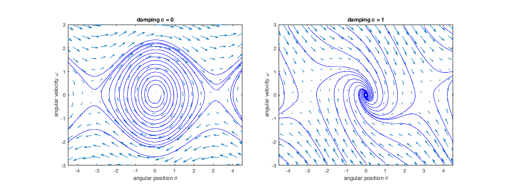
Example:

The motion of a simple pendulum can be described by the following second-order ODE:

$$\theta''+c\theta'+\frac{g}{L}\sin\theta=0$$ (169)

where $c$ is the damping coefficient, $L$ is the length of the support rod, and $g$ is gravitational acceleration. This nonlinear ODE can be linearized if we can assume the angle $\theta$ is small, and consider the Maclaurin expansion of $\sin\theta$:

$$\sin\theta=\sin(0)+\sin'(0)\theta+\frac{1}{2}\sin''(0)\theta^2+\cdots \approx \sin'(0)\theta=\cos(0)\theta=\theta$$ (170)

and we get a LCCODE

$$\theta''+c\theta'+\frac{g}{L}\theta=0$$ (171)

This second order ODE can be converted into two first-order ODEs

$$\left\{\begin{array}{ccl}\theta'&=&\omega\\ \omega'&=&-c\,\omega-g\sin\theta/L \end{array}\right.$$ (172)

or in vector form:

$${\bf y}'=\left[\begin{array}{c}\theta\\ \omega\end{array}\right]'... ...ft[\begin{array}{l}f_1=\omega\\ f_2=-c\,\omega-g\sin\theta/L \end{array}\right]$$ (173)

The equilibrium point satisfies

$$\theta' = \omega=0$$

$$\omega' = -c\,\omega-g\cos\theta/L=0$$ (174)

From the second equation we get $\sin\theta=0$, i.e., there are two equilibrium points ${\bf y}^*_1=(\theta=0,\;\omega=0)$ and ${\bf y}^*_2=(\theta=\pi,\;\omega=0)$. In the neighborhood of the equilibrium point ${\bf y}^*$ satisfying ${\bf y}'={\bf f}({\bf y}^*)={\bf0}$, we have

$${\bf y}' \approx {\bf J}_f{\bf y}=\left[\begin{array}{cc} \frac{\... ...right] =\left[\begin{array}{cc} 0 & 1 \\ -g\cos\theta/L & -c \end{array}\right]$$ (175)

Consider the two cases:

• $\theta=0$, $\cos\theta=1$:

  $$\lambda_{1,2}=\frac{1}{2}\left(-c\pm\sqrt{c^2-4g/L}\right)$$ (176)

  If $c=0$, both eigenvalues $\lambda_{1,2}=\pm j\sqrt{g/L}$ are purely imaginary, the motion is a sinusoidal oscillation; if $c>0$, $\lambda_{1,2}<0$, the motion is an attenuated oscillation.

• $\theta=\pi$, $\cos\theta=-1$:

  $$\lambda_{1,2}=\frac{1}{2}\left(-c\pm\sqrt{c^2+4g/L}\right)$$ (177)

  One of the eigenvalues is positive while the other negative (saddle point), the solution is unstable.

The phase planes of the pendulum problem corresponding to $c=0$ and $c=1$ are shown below. We see that the equiliburim point $(\theta,\;\omega)=(0,\;0)$ is stable while the equiliburim point $(\theta,\;\omega)=(\pi,\;0)$ is unstable (saddle point).

We next consider the complete solution of a second order LCCODE in the following canonical form:

$$y''(t)+2\zeta\omega_n y'(t)+\omega_n^2 y(t)=x(t)$$ (178)

Same as in the first order case, the complete solution of this second order LCCODE is composed of the homogeneous solution $y_h(t)$ when $x(t)=0$, and the particular solution $y_p(t)$ when $x(t)\ne 0$.

In the following, we will first consider various methods for solving first-order ODEs, and then extend such methods to solving first order ODE systems containing multiple ODEs $y'_i(x)=f_i(x,\,y_1(x),\cdots,y_N(x))\;\;(i=1,\cdots,N)$, and higher order ODEs $y^{(N)}(x)=f(x,\,y'(x),\cdots,y^{(N-1)}(x))$.